2080
IEEE JOURNAL OF SELECTED TOPICS IN APPLIED EARTH OBSERVATIONS AND REMOTE SENSING, VOL. 7, NO. 6, JUNE 2014
Dynamic Linear Classifier System for Hyperspectral Image Classification for Land Cover Mapping Bharath Bhushan Damodaran and Rama Rao Nidamanuri
Abstract—Exploitation of the spectral capabilities of modern hyperspectral image demands efficient preprocessing and analyses methods. Analysts’ choice of classifier and dimensionality reduction (DR) method and the harmony between them determine the accuracy of image classification. Multiple classifier system (MCS) has the potential to combine the relative advantages of several classifiers into a single image classification exercise for the hyperspectral image classification. In this paper, we propose an algorithmic extension of the MCS, named as dynamic classifier system (DCS), which exploits the context-based image and information class characteristics represented by multiple DR methods for hyperspectral image classification for land cover mapping. The proposed DCS algorithm pairs up optimal combinations of classifiers and DR methods specific to the hyperspectral image and performs image classifications based only on the identified combinations. Further, the impact of various trainable and nontrainable combination functions on the performance of the proposed DCS has been assessed. Image classifications were carried out on five multi-site airborne hyperspectral images using the proposed DCS and were compared with the MCS and SVM based supervised image classifications with and without DR. The results indicate the potential of the proposed DCS algorithm to increase the classification accuracy considerably over that of MCS or SVM supervised image classifications. Index Terms—Dynamic classifier system (DCS), ensemble classification, hyperspectral image, land cover classification, multiple classifier system (MCS), remote sensing, supervised learning.
I. INTRODUCTION YPERSPECTRAL image classification suffers from the curse of high dimensionality popularly known as Hughes phenomena [1]. Dimensionality reduction (DR) methods mitigate this problem and make possible the application of classical statistical supervised classifiers on hyperspectral image. A number of DR methods and classifiers are proposed in literature for hyperspectral image classification. However, the performance of a DR method depends upon the nature of information classes and the classifier used [2], [3]. Thus, the classification accuracy depends upon the subjective choice of DR methods and classifiers. Identifying an optimal pair of DR method and classifier is a tedious task; given the numerous possibilities in classifiers, DR methods, and the nature and distributions of information classes.
H
Manuscript received February 28, 2013; revised November 22, 2013; accepted November 29, 2013. Date of publication January 08, 2014; date of current version August 01, 2014. The work of B. B. Damodaran was supported by a Doctoral Fellowship provided by the Indian Institute of Space Science and Technology, Department of Space, Government of India. The authors are with the Department of Earth and Space Sciences, Indian Institute of Space Science and Technology, Thiruvananthapuram, Kerala 695 547, India (e-mail:
[email protected];
[email protected]). Color versions of one or more of the figures in this paper are available online at http://ieeexplore.ieee.org. Digital Object Identifier 10.1109/JSTARS.2013.2294857
Numerous studies have addressed the suitability of DR methods and classifiers for different applications and have suggested particular classifier and/or DR method appropriate for that particular application [3]–[6]. A common observation of these studies is that the selection of DR methods for the application at hand has to be done in relation with the classifier to be used. Most of the studies report optimal classifiers for specific applications and conclude that the classifier selection is a function of DR method. This context-specific knowledge may not be applicable across different hyperspectral images and applications. A multiple classifier system (MCS), an advanced pattern recognition technique, is emerging [7]–[9] as an alternative paradigm for image classification to avoid the need of determining optimal classifier for each and every image analysis task a priori. An MCS permits simultaneous application of several classifiers on the input data, and the intermediate outputs of all the classifiers are combined for producing the final classified image. Most of the MCS architectures reported in the literature are designed to provide different input data sources to same classifier or same input data source to different classifiers [7], [10], [11]. When the same input data are given to different classifiers, there could be an overlap in the decision boundaries of the classifiers [12]. Moreover, recently, it has been reported that there are no significant accuracy differences among most of the commonly used classifiers at the overall image level, but significant differences in perclass accuracy for some information classes [3], [13]. In other words, certain type of information classes prefer certain type of classifiers and DR methods for better discrimination. This indicates the importance of selecting classifiers and DR methods in relation to information content of hyperspectral image. Maintaining diversity in the classifiers and choosing appropriate combination scheme are vital to the functioning of the MCS. A major limitation of the MCS is that, without addressing the input data dynamics, merely inclusion of the classifiers of divergent groups may not necessarily yield the results expected from the MCS; instead end up producing results which are inferior to that of classical supervised classification [14], [15]. Most of the literature on MCS deal with innovations in combination function schemes and creating diversity using different simple classifiers [11], [16]. The extension of the MCS framework to let it acquire the capability to dynamically identify optimal pairs of DR methods and classifiers simplifies image classification and reduces the data and application dependence of the MCS. Further, our literature review reveals that the potential of creating diversity in the MCS based on differential performances of various classifiers against different DR methods has not been addressed. The creation of diversity in the classification process by deploying multiple DR methods is, in principle,
1939-1404 © 2014 IEEE. Personal use is permitted, but republication/redistribution requires IEEE permission. See http://www.ieee.org/publications_standards/publications/rights/index.html for more information.
DAMODARAN AND NIDAMANURI: DYNAMIC LINEAR CLASSIFIER SYSTEM FOR HYPERSPECTRAL IMAGE CLASSIFICATION
possible as each different DR method generates data variance characteristic to its formulation and the distinct way of transformation. The objective of this work was to develop an algorithm, we label as dynamic classifier system (DCS), to dynamically select optimal pairs of classifiers and DR methods from a pool of classifiers and DR methods for hyperspectral image classification for land cover mapping. Further, the comparative performance of various trainable and nontrainable combination functions for combining the decision function values of the DCS has been assessed. The proposed DCS method is aimed at reducing the extensive human expert involvement in the selection of classifiers and DR methods in supervised image classification for various land cover mapping scenarios. The proposed DCS was designed with five DR methods and seven classifiers and was implemented for the classification of five multi-site multi-sensor airborne hyperspectral images for the discrimination of a range of land cover classes.
II. METHODOLOGY A. DR Methods We provide a brief description of the DR methods used for generating different variants of the input hyperspectral image in the MCS. The popular DR methods—principal component analysis (PCA), independent component analysis (ICA) [5], minimum noise fraction (MNF) [17], kernel principal component analysis (KPCA) [18], and discrete wavelet transform-based dimensionality reduction (DWT-DR) method [19]—were used to transform the hyperspectral images in to low dimensional space. The PCA, MNF, ICA, and KPCA are based on statistical transformations which project data on to a new coordinate system by maximizing or minimizing certain statistical measures. The PCA and MNF maximize the second-order statistics (variance) in the projected components. The eigen vectors of the covariance matrix are used as the basis for the transformation, and eigen values of the covariance matrix represents variance along each projected direction. The higher-order statistics are used as the measures by ICA to maximize the nonGaussianity in the projected components. The PCA and MNF result in orthogonal components, whereas ICA results in independent components. The choice of ICA is more effective when the extent of materials present in the scene is relatively small [5]. The KPCA is an extension of the PCA in which the input data points are transformed to higher-dimensional space (called as feature space) by a nonlinear transformation. In the feature space, the KPCA performs similar to the linear PCA. The KPCA has the advantage of capturing the higher-order statistics and provides better separability of the classes over the linear PCA [18]. The wavelet transform is an effective tool extensively used in signal and image processing. The basis for the wavelet transform is fixed unlike statistical transformation. Each pixel in the hyperspectral image was decomposed by the wavelet transform using Daubechies filter (DB6). The outlier in the image was discarded and the approximation coefficients were reconstructed using inverse discrete wavelet transform. The required level (L) of decomposition could be decided based on the acceptable correlation between the decomposed signal and the original
2081
signal [19]. In this work, we generated series of wavelet transformed hyperspectral image with different level of decompositions. B. Classifiers Used in MCS A set of simple classifiers with linear decision boundary, which can be broadly categorized into spectral matching methods, probabilistic methods, and subspace modeling methods, were selected for designing the MCS. The advantage of these methods is its fast training performance, since it requires only calculating mean of each class and common covariance matrix of the training samples. We give below a brief description of the classifiers selected. 1) Spectral Matching Methods: The spectral matching-based methods consist of minimum distance classifier (MDC) [21] and spectral similarity measure (SSM) [22]. The MDC labels an unknown pixel based on the minimum distance criterion. The SSM labels the pixels based on spectral angle and spectral brightness differences between the image and reference pixels. These classifiers label the unknown pixel based on the minimum decision function value. 2) Probabilistic Methods: The probabilistic methods consist of linear discriminant classifier (LDC), logistic regression classifier (LRC), and naive Bayes classifier (NBC). The LDC can be derived from the maximum-likelihood classifier (MLC). An MLC assumes that the classes are normally distributed with different mean and covariance. It becomes LDC, under the condition that all the classes have equal co-variance [23]. An NBC assumes that the features of input data are linearly independent and normally distributed. It estimates the parameters (mean and variance) along each feature and finds the likelihood for each of the features in the input data. Since the features are independent, the posterior probabilities are estimated by taking the product of the likelihood of each of the features and prior probability [24]. An LRC is a binary classifier which linearly weights the input data features, and the weights are obtained by maximizing the log-likelihood function through maximum-likelihood estimate. Then, the sigmoid function is applied over the weighted sum of the input features. For multiclass problem, the logistic regression is implemented by one strategy versus rest strategy [24], [25]. This group of classifiers labels unknown image pixel based on the maximum posterior probability values. 3) Subspace Modeling Methods: The subspace modeling methods consist of orthogonal subspace projection (OSP) and target-constrained interference minimized filter (TCIMF). These methods work based on nullifying the undesired and interfering class members. The OSP assumes the hyperspectral pixel vector as a linear combination of a set of finite class members present in the image. It divides the class mean matrix into desired class mean (any one of the class) and undesired class mean matrix (remaining classes). The goal of OSP is to find an orthogonal complement projector for each of the desired class (one at time) which projects the unknown pixel into a subspace orthogonal to the undesired class mean matrix [26]. The unknown pixel is assigned to the class which has maximum decision value. The TCIMF is an extension of the constrained energy minimization algorithm. It assumes that the hyperspectral pixel vector is made
2082
IEEE JOURNAL OF SELECTED TOPICS IN APPLIED EARTH OBSERVATIONS AND REMOTE SENSING, VOL. 7, NO. 6, JUNE 2014
up of three separate sources such as desired pixel vector, undesired pixel vectors, and interference. Similar to OSP, the TCIMF also splits the class mean vectors into desired class and undesired class mean vectors. It is designed by the finite impulse response (FIR) filter that passes the desired class mean vector, while annihilating the undesired class mean vectors. The weight vector of FIR filter for each of the desired class is computed by minimizing the energy of the filter [27]. These methods label unknown image pixel based on the maximum decision function value. C. Diversity Measurement Diversity among the classifiers set is important when constructing an MCS. However, quantitative description of the diversity is not straight forward and there is no accepted formal definition. Further, there is no direct relationship between the diversity and accuracy of the MCS [28]. To quantify the diversity introduced by deploying hyperspectral image after applying the DR methods, we adopted two statistical diversity measures: disagreement measure (DM) [29] and Kohavi–Wolpert variance measure (KWM) [30] which belong to pairwise and nonpairwise categories of diversity measures, respectively. The DM is the ratio between the number of samples on which one classifier is correct and other is incorrect to the total number of samples. Suppose there are classifiers, then the averaged pairwise DM is given by
where is the number of samples correctly classified by th classifier and incorrectly classified by the th classifier, is the number of samples correctly classified by th classifier and incorrectly classified by the th classifier, and is the total number of samples. Similarly, the Kohavi–Wolpert measure is given by
where is the total number of samples and is the number of classifiers which correctly classify the th sample. The diversity increases with increasing values of DM and KWM. In principle, any one of the diversity measures can be used for quantifying the diversity. However, a combination of these two categories of measures provides complimentary characteristics of diversity as both of them can be linearly related. Hence, the total diversity measure (DA) of the set of classifiers in the MCS can be calculated from (1) and (2) as
D. Approach for Introducing Dynamic Selection of Classifiers in MCS In a typical MCS application, all the classifiers forming the classifiers set are applied on the input data irrespective of the inherent data dynamics with reference to the classifiers set. This
structural constraint of the MCS may lead to poor classification performance and end up being no better than the classification performance achieved in a typical supervised image classification. We redesigned the MCS framework to automatically select and execute pairs of classifiers and DR methods which are compatible and offer optimal results. be the set of classifiers, Let be the set of DR methods, is the number of test pixels drawn from the classified image, and is the number of categories in the classified image, then the error matrix can be expressed as the distribution of test pixels into cells. Let denote the number of test pixels classified into category in the classified image of category in the reference pixels, and let and
are the row and column sums of the error matrix
, respectively. Then, the overall accuracy can be computed as . Similarly, producer’s accuracy (P) and user’s accuracy (U) can be computed as and , respectively. The kappa coefficient is calculated as
These intermediate accuracy estimates were used for estimating the optimal dimensionality and pairing up the classifiers and dimensionality methods by classifying the training pixels by all the classifiers and DR methods. Apart from this approach, the optimal dimensionality of DR methods can also be estimated by using a class separability measure which has computational advantage. Hence, the proposed DCS has also been implemented to obtain the optimal dimensionality of hyperspectral image, which is independent of the classifier by a class separability measure, Jeffreys–Matusita (JM) distance measure extended for multiclass category, and is equivalent to Bhattacharya bound [20]. As the JM distance measure is a monotonic function, the flattening point of the curve is selected as the optimal dimension of the DR methods. The performance of the proposed DCS with these two approaches was compared. Fig. 1 depicts the schematic outline of the proposed DCS with three stages and the algorithmic development of the DCS is shown in Fig. 2. Stage I involves 1) constructing the pool of DR methods and classifiers and 2) finding the optimal dimension of DR methods relative to each classifier. In stage II, the MCS was programmed to select an optimal classifier relative to each DR method based on the classification accuracy estimates of training samples and the class separability measure while considering the diversity score. By this stage, the anticipated advantage is to give the MCS the ability to select only a subset of classifiers and corresponding DR methods for further processing for producing final classification results. In the present case, the MCS identifies five pairs of classifier and DR method which are accurate and diverse for further processing. The relative merits of identified classifier relative to each DR method are combined together in
DAMODARAN AND NIDAMANURI: DYNAMIC LINEAR CLASSIFIER SYSTEM FOR HYPERSPECTRAL IMAGE CLASSIFICATION
2083
Fig. 1. Schematic outline of the proposed DCS. In Stage I, the image classifications with all the classifiers relative to each DR method are performed. In Stage II, the DCS identifies pairs of optimal classifier and DR method. In Stage III, the output from the pairs of classifiers and DR method are combined to obtain final classified image.
Fig. 2. Algorithmic representation of the proposed DCS.
2084
IEEE JOURNAL OF SELECTED TOPICS IN APPLIED EARTH OBSERVATIONS AND REMOTE SENSING, VOL. 7, NO. 6, JUNE 2014
NUMBER
OF
TABLE I REFERENCE DATA SAMPLES
stage III to produce final classified image. We label this modified version of the MCS in which the classifiers are selected adaptive to specific image data at hand as “DCS.” Irrespective of the sophistication and suitability of the classifiers and corresponding DR methods, the image classification results are ought to be influenced by the combination function used [8], [12]. It is, therefore, desirable to have an idea of the impact of various combination functions on the proposed DCS. E. Evaluation of Classifier Combination Functions As is the case with MCS, the performance of the proposed DCS depends upon the type of combination function adopted for combining the intermediate classified images. It is, therefore, necessary to assess the impact of various combination functions on the performance of the proposed DCS. As the classifiers considered in the MCS are heterogeneous, the classifiers’ decision values have to be transformed into a common scale before combining the classifiers. Let be the decision values of the classifier for classes, then decision values of the classifier can be transformed as follows: shown in the equation at the bottom of the page. After the above transformation, the selected classifiers relative to each DR method were combined by six nontrainable combination functions and two trainable combination functions. The nontrainable combination functions are majority voting (MV), maximum rule (max), minimum rule (min), product rule (prod), average rule (avg), and median rule (med). These combination functions have been extensively used in MCS due to their simplicity and robustness [11]. In the trainable combination functions, we used supervised classifiers namley, support vector
machines (SVM) and MLC. The decision function values of the classifiers in the DCS are stacked together as a 1-D vector and fed as the input to the trainable combination function [7], [31]. If there are classifiers and number of classes, then , is the decision function value of th classifier and th class. Then, the decision function values of classifiers are stacked together as , where element in is a vector consisting of classifiers decision values for classses. F. Image Classification Using MCS and SVM In order to assess the comparative performance of the proposed DCS with the state-of-the-art methods, all the five hyperspectral images were classfied by the MCS and SVM using the same reference data samples. Because the SVM and some of the classifers in the MCS can classify high dimensionality data even without DR, we performed the image classification experiments with and without DR for all the combination functions. The SVM classification is performed with RBF kernel using LIBSVM [32]. Grid search method has been used to determine the optimal parameters of the SVM. The best classification accuracies were retained for comparison with the DCS. G. Validation of the Results All the classified images were validated by cross-validation [33] to obtain robust estimates of accuracies of the classification experiments. All the reference data were split into training (90%) and testing (10%) samples by 10-fold cross-validation and then performed classification of each image 10 times for the possible 10 splits. For each classified image, an error matrix, overall
DAMODARAN AND NIDAMANURI: DYNAMIC LINEAR CLASSIFIER SYSTEM FOR HYPERSPECTRAL IMAGE CLASSIFICATION
2085
Fig. 3. False color composites of hyperspectral images: (a) ROSIS image of University of Pavia, Italy; (b) ROSIS image of part of the city of Pavia, Italy; (c) ProSpecTIR image of part of Reno, NV, USA; (d) HyMAP image of Dedelow, Germany; and (e) HYDICE image of part of Washington DC, USA.
accuracy, and kappa coefficient were calculated. The accuracy estimates thus obtained were averaged to obtain representative accuracy and error estimates. The number of reference data samples used is shown in Table I. Further, the statistical significance of the differences among the different classification results was assessed by Z-test [34] and McNemar test (Chi-squared test) [35] at 95% of confidence interval.
III. RESULTS AND ANALYSIS A. Hyperspectral Datasets Experiments were performed on five different hyperspectral images which represent diverse land cover categories in agriculture, urban, and mixed environmental settings. 1) HyMAP Image: The HyMAP hyperspectral image was collected over the Dedelow research station of the Leibniz— Centre for Agricultural Landscape Research (ZALF), Germany by the DLR (German national aerospace agency). The
predominant land-use categories in the study site are agricultural crops namely, wheat, winter rape, winter wheat, built up, and grass. The image has a spatial resolution of 5 m and 128 spectral bands with spectral resolution up to 20 nm in the spectral range of . A subset of the image acquired was used in this study. 2) ROSIS Image: The ROSIS hyperspectral dataset consist of two images collected over the University of Pavia and the part of the city of Pavia, Italy, by the ROSIS airborne hyperspectral sensor in the framework of HySens project managed by DLR (German national aerospace agency). The ROSIS sensor collects images in 115 spectral bands in the spectral range of with spatial resolution of 1.3 m. The image collected over the University of Pavia is named as ROSIS University image and consists of 10 land cover classes namely, trees, asphalt, meadow, gravel, metal sheet, bare soil, bitumen, bricks, shadows, and built up. The image collected over the city of Pavia is named as ROSIS city of Pavia image and consists of 10 land cover classes namely water, trees, asphalt,
2086
IEEE JOURNAL OF SELECTED TOPICS IN APPLIED EARTH OBSERVATIONS AND REMOTE SENSING, VOL. 7, NO. 6, JUNE 2014
IDENTIFIED PAIRS
OF
OPTIMAL CLASSIFIER
AND
DR METHOD
TABLE II PROPOSED DCS AND THE CORRESPONDING BEST CLASSIFICATION ACCURACY
BY THE
OA, overall accuracy; KC, kappa coefficient. Estimated optimal dimension of DR method is in brackets.
meadow, self building blocks, tiles, bare soil, bitumen, shadows, and built up. 3) ProSpecTIR Urban and Mixed Environment Image: The ProSpecTIR airborne hyperspectral image was collected over part of the city of Reno, NV, USA. This image consists of 356 spectral bands in the spectral range of with spatial resolution of 1 m. The dominant land-use categories in this image are trees, water, bare soil, asphalt, built up, shadows, and vehicles. 4) HYDICE Image: This airborne hyperspectral image was collected over a mall in Washington DC, USA, at 2-m spatial resolution by the HYDICE airborne hyperspectral sensor. This image consists of 191 bands in the spectral range of . The prominent land-use categories are roof, grass, trees, path, road, shadow, and water. False color composites of the hyperspectral images are shown in Fig. 3. B. Dynamic Selection of Classifiers Relative to DR Methods by the Proposed DCS For each DR method, one optimal classifier was identified from the pool of classifiers by 1) DCS constructed with the accuracy estimates obtained from the classification of training samples [Table II(a)] and 2) DCS constructed with class separability measure [Table II(b)]. The estimated optimal dimension of the DR methods is indicated in brackets. It can be observed that the DCS identified different classifiers for different DR methods. The comparison of classifiers identified from the pool of classifiers reveals that only one classifier is repeated twice for different hyperspectral images. Further, an examination for repetition of the optimal classifiers for multiple hyperspectral images which contain similar land covers indicates significant variations with respect to DR methods. This indicates that the optimal classifier identified from a particular hyperspectral image need not necessarily be applicable to another similar type of hyperspectral image, thus emphasizing the need for adaptive selection of classifiers. The comparison between Table II(a) and (b) indicates that the classification accuracies of the best classifier and DR pair are not highly variable across different
hyperspectral images despite the occurrence of different classifiers as optimal. Frequency of the selected classifiers by the DCS relative to different DR methods and hyperspectral images indicates that some classifiers are most selected, whereas few classifiers are least selected. These observations highlight the potential of DCS to avoid influence of unsuitable classifiers in image classification. C. Impact of the Combination Function on the Classification Performance of the Proposed DCS In principle, the classified image obtained from any one of the pairs of classifiers and DR methods identified by the DCS could be the final classified image for land cover mapping. However, running the DCS unrestricted leads to performing classification using all the pairs of optimal classifiers and DR methods for the same hyperspectral image; this results in multiple classified images with variations in the classification accuracy, however, marginal. Within the framework of the proposed DCS, we assessed the possibility of further enhancement of classification accuracy by combining the classified images obtained from the multiple pairs of classifiers and DR methods using several trainable and nontrainable combination functions. The overall accuracies and kappa coefficient are presented in Table III(a) (for DCS with optimal dimensionality estimated by training samples classification) and Table III(b) (for DCS with optimal dimensionality estimated by class separability measure) and the corresponding classified images with best combination functions in Figs. 4(A), (B), and 5(A), (B). 1) DCS With Nontrainable Combination Function: The performance of proposed DCS changed considerably with different nontrainable combination functions. When compared with the best classifier and DR pair (see Table II), there has been marginal to significant increase in the overall accuracy. Table III(a) shows the classification accuracy obtained by the DCS combination function, when the optimal dimension of the DR methods are determined by the classification accuracy of the training samples. The classification accuracy increased by 4.09% and 5.22% with average rule and majority voting rule for
DAMODARAN AND NIDAMANURI: DYNAMIC LINEAR CLASSIFIER SYSTEM FOR HYPERSPECTRAL IMAGE CLASSIFICATION
2087
Fig. 4. (A) DCS-based classified images (best nontrainable combination function; the optimal dimension of the DR methods was estimated based on training samples classification): (a) ROSIS University, (b) ROSIS City of Pavia, (c) ProSpecTIR, (d) HyMAP, and (e) HYDICE. (B) DCS-based classified images (best nontrainable combination function; the optimal dimension of the DR methods was estimated based on class separability measure): (a) ROSIS University, (b) ROSIS City of Pavia, (c) ProSpecTIR, (d) HyMAP, and (e) HYDICE.
2088
IEEE JOURNAL OF SELECTED TOPICS IN APPLIED EARTH OBSERVATIONS AND REMOTE SENSING, VOL. 7, NO. 6, JUNE 2014
Fig. 5. (A) DCS-based classified images (best trainable combination function; the optimal dimension of the DR methods was estimated based on training samples classification): (a) ROSIS University, (b) ROSIS City of Pavia, (c) ProSpecTIR, (d) HyMAP, and (e) HYDICE. (B) DCS-based classified images (best trainable combination function; when the optimal dimension of the DR methods was estimated based on class separability measure): (a) ROSIS University, (b) ROSIS City of Pavia, (c) ProSpecTIR, (d) HyMAP, and (e) HYDICE.
DAMODARAN AND NIDAMANURI: DYNAMIC LINEAR CLASSIFIER SYSTEM FOR HYPERSPECTRAL IMAGE CLASSIFICATION
TABLE III CLASSIFICATION RESULTS FROM DCS (OPTIMAL DIMENSIONS OF THE DR METHOD WERE ESTIMATED BASED ON TRAINING SAMPLES CLASSIFICATION AND CLASS SEPARABILITY MEASURE)
2089
TABLE IV STATISTICAL SIGNIFICANCE TEST [Z-TEST AND MCNEMAR TEST (CHI-SQUARED TEST)] BETWEEN DCS AND SINGLE BEST CLASSIFIER AND DR METHOD PAIR FOR ALL THE COMBINATION FUNCTIONS (OPTIMAL DIMENSIONS OF DR METHOD WERE ESTIMATED BASED ON TRAINING SAMPLES CLASSIFICATION AND CLASS SEPARABILITY MEASURE)
The statistically significant cases are highlighted in bold.
Overall accuracy (OA, in %) and kappa coefficient (KC) of the classified image obtained by the combination of the optimal pairs of classifiers and DR methods for various combination functions.
HyMAP and HYDICE hyperspectral images, respectively. For ROSIS University, ProSpecTIR, and ROSIS City of Pavia hyperspectral images, the classification accuracy improved by 5.46%, 5.42%, and 3.59% with product rule, respectively. The classification accuracy of the combination functions, when the optimal dimension of the DR methods was estimated by the class separability measure, is shown in Table III(b). The magnitude of increase in classification accuracy is similar to Table III(a) for ROSIS City of Pavia and HYDICE hyperspectral images. For remaining hyperspectral images, the increase in classification accuracy is less than one order of magnitude over the best classifier and DR pair. From Table III, it can also be inferred that there is more than one nontrainable combination functions which offer better classification accuracy with all the five hyperspectral images. Moreover, the product and average rule resulted in similar classification accuracy for all the five hyperspectral images. The DCS-based classification using maximum and minimum as the combination function resulted in accuracy either decreased or no change to the best classifier and DR pair for some of the hyperspectral images. This observation suggests the significance of the adopting appropriate combination function to fully exploit the potential of DCS. 2) DCS With Trainable Combination Function: When the intermediate classified images in the DCS were combined with trainable combination functions, the classification accuracy increased further when compared with the results obtained from the nontrainable combination functions. From Table III (a), the classification accuracy of the DCS (when the optimal
dimension of the DR methods was estimated based on classification accuracy of training samples) with the SVM combination scheme is increased by 6.60%, 9.59%, 6.43%, 5.65%, and 4.99% for the HyMAP, ROSIS University, ProSpecTIR, ROSIS City of Pavia, and HYDICE hyperspectral images, respectively. With the MLC combination scheme, the classification accuracy has improved up to 6% for ROSIS University and HYDICE images and 2%–4% for the remaining hyperspectral images. The combination of selected classifiers by the DCS (when the optimal dimension of the DR methods was estimated based on class separability) in Table II(b) has resulted in 3%–9% improvement with the SVM combination scheme and 3%–6% of improvement with the MLC combination scheme. Compared to Table III(a), there is a similar magnitude of improvement in the classification accuracy for the three images and negligible magnitude difference (1%) for the remaining images. However, the classification accuracies resulted in Table III(a) are higher for the four hyperspectral images compared to Table III(b). Contrary to this, Table III(b) results in higher classification accuracy for ProSpecTIR hyperspectral image. The results of the statistical significance test are shown in Tables IV–VI. Under the condition > and > , the difference in accuracy is regarded as statistically significant at 95% confidence interval. The statistically significant cases are highlighted in bold. As evident from Table IV, the accuracy differences between the single best classifier/DR pair and the DCS are significant for most of the combination functions. A significant increase in the classification accuracy has been observed with all the five hyperspectral images. However, the accuracy differences amongst the nontrainable combination functions are marginal to moderate. When compared to nontrainable combination functions, the accuracy improvements by DCS with trainable combination function are consistently higher by magnitude and are statistically significant for four of the five hyperspectral images (see Table V and VI).
2090
IEEE JOURNAL OF SELECTED TOPICS IN APPLIED EARTH OBSERVATIONS AND REMOTE SENSING, VOL. 7, NO. 6, JUNE 2014
TABLE V STATISTICAL SIGNIFICANCE TEST (Z-TEST AND MCNEMAR TEST (CHI-SQUARED TEST)) BETWEEN DCS AND SINGLE BEST CLASSIFIER AND DIMENSIONALITY REDUCTION METHOD PAIR FOR ALL THE COMBINATION FUNCTIONS (OPTIMAL DIMENSION OF DIMENSIONALITY REDUCTION METHOD WAS ESTIMATED BASED ON CLASS SEPARABILITY MEASURE)
TABLE VI STATISTICAL SIGNIFICANCE TEST [Z-TEST AND MCNEMAR TEST (CHI-SQUARED TEST)] BETWEEN THE BEST NONTRAINABLE COMBINATION FUNCTION AND THE TRAINABLE COMBINATION FUNCTION OF THE DCS
The statistically significant cases are highlighted in bold.
TABLE VII CLASSIFICATION ACCURACY (%) OBTAINED WITH MCS (WITH BEST COMBINATION FUNCTION), SVM (WITH AND WITHOUT DR METHOD), THE PROPOSED DCS (WITH THE BEST COMBINATION FUNCTION), AND THE BEST CLASSIFIER/DR PAIR The statistically significant cases are highlighted in bold.
D. Comparison of Classification Performance of the Proposed DCS With MCS and SVM Table VII shows the overall accuracy estimates obtained from SVM, MCS, and DCS for all the five images. For reference, the overall accuracy obtained with the best classifier/DR pair is also included. Table VII(a) shows the accuracies offered by the DCS (the optimal dimension of the DR methods was estimated based on the training samples classification) when combining the selected classifier and DR pair in Table II(a). The DCS offered consistently higher accuracies when compared with the MCS or SVM methods, even though with relatively lower margin for HYDICE image. The DCS shows 3.2%, 7.16%, 2.42%, 4.52%, and 2.79% increase when compared with MCS and 3.94%, 4.39%, 1.9%, 3.51%, and 2.86% increase when compared with SVM for the HyMAP, ROSIS University, ProSpecTIR, ROSIS City of Pavia, and HYDICE image, respectively. When the pair of classifiers and DR method resulted in Table II(b) are combined, the DCS offers about 4%–6% enhancement in classification accuracy over the MCS and about 2% improvement over the SVM classification. Further, the drastic enhancement in classification accuracy of DCS, an increase of about 11%–13%, can be observed when compared with SVM and MCS classification without DR method in Table VII(a) and (b). The comparison between Table VII(a) and (b) shows that there is about 2% accuracy difference for HyMAP, ROSIS University, and ROSIS City of Pavia hyperspectral images and for the remaining images, the accuracies are comparable. Table VII indicates that SVM’s performance is comparable or better than the MCS when applied with DR: out of the five images, SVM offered marginally higher accuracy for three images; whereas the MCS indicates marginal increase for two images. However, the performance of SVM and MCS varied significantly while implementing with and without applying DR. These observations conclude that DCS is a good candidate to produce diverse and adaptive classifiers in the MCS for hyperspectral image classification.
E. Computational Complexity Analysis Table VIII shows the computational complexity analysis of the DCS and MCS. The MCS combines all the classifiers relative to each DR method, whereas the DCS combines only the identified optimal classifier relative to each DR method. It is interesting to observe that the computation time of DCS is better than the MCS with single DR method and with all the five DR methods. This may be due to the computational time difference of the SVM combination function in MCS and DCS. In the MCS, all the classifiers are engaged in the combination function, which gets further complicated by the use of the SVM combination function. In the DCS, only a subset of the classifiers is engaged in the combination function, thereby compensating the computational complexity introduced by the dynamic selection criteria. The computation time mentioned in Table VIII is calculated for 10 runs and it includes both training and testing time. The experiments are performed with a typical desktop computer (4 GB RAM, Intel i-5 processor @ 3.20 GHz, 64-bit operating system), and it has been observed that the computational time for the selection of the optimal classifiers and DR methods in the DCS is 1 s. The computation time of DCS with optimal dimensionality estimated by training samples classification and class separability measures
DAMODARAN AND NIDAMANURI: DYNAMIC LINEAR CLASSIFIER SYSTEM FOR HYPERSPECTRAL IMAGE CLASSIFICATION
COMPUTATION TIME (CPU TIME
IN
S) TAKEN
BY THE
DIVERSITY ESTIMATES
TABLE VIII MCS WITH ALL THE DR METHODS, MCS WITH SINGLE DR METHOD, AND
OF THE
2091
THE
PROPOSED DCS
TABLE IX MCS AND DCS FOR THE HYPERSPECTRAL IMAGES CONSIDERED
differed considerably with the class separability measure showing relatively better performance. However, the apparent computational comparisons are variable by the number of information classes in the hyperspectral image.
The analysis of the diversity measures shows that there is a positive relationship between diversity and classification accuracy. For example, the DCS offered highest increase in the accuracy for ROSIS University image for which the diversity measures show highest magnitudes.
F. Diversity Creation in the MCS With Multiple DR Methods The statistical diversity measures, DM and KWM, were applied on the MCS to quantify the diversity existed in the MCS with and without DR methods. Table IX shows the computed DM and KWM values for the various hyperspectral images. The DM and KWM values for each hyperspectral image without DR are the diversity existed in the classifiers considered for designing the MCS. As seen in Table IX, the diversity estimate increased considerably after the DR methods were applied. Further, diversity in MCS is considerably higher when the optimal dimension of the DR methods was determined by class separability measure [see Table IX(b)]. The change in diversity values across different images indicates the inherent differences in the data acquired from different sources and environmental conditions.
IV. DISCUSSION Hyperspectral remote sensing data has been emerging as the standard data source for land cover classification, target identification, and thematic mapping from local to regional scales. However, the high dimensionality of the hyperspectral data confounded by spectral correlation poses challenges to process for meaningful exploitation of its capabilities. The classical image classification techniques are exposed with new challenges in terms of data dimensionality, limited training samples, and to cater to the needs of wider application domains [36], [37]. Consequently, a number of DR methods and classifiers have been developed. However, there is no classifier or DR method which is optimal across hyperspectral data sources and
2092
IEEE JOURNAL OF SELECTED TOPICS IN APPLIED EARTH OBSERVATIONS AND REMOTE SENSING, VOL. 7, NO. 6, JUNE 2014
application domains. In general, the appropriate classifier and DR method are identified before hand by analyst’s prior knowledge or on heuristic basis, thus making the results being subjective and the procedure being expert dependent. There has been an increasing interest in the development of methods for efficient classification of hyperspectral image. An MCS is viewed as one of the effective methodologies to improve hyperspectral image classification performance [8], [9], [31], [38]. During the last two decades, MCS has developed significantly by theories and empirical studies and has been used widely in various applications of pattern recognition. The necessity of generating multiple transformations of image and selection of appropriate classifier from a pool of classifiers for hyperspectral image classification can be easily handled by the MCS architecture. However, the success of MCS depends upon the diversity of classifiers’ performance [7], [11]. In principle, different variants of a hyperspectral image can be generated by using different DR methods and the set of all these images can then be exploited for diversity requirement in the MCS. Our results indicate that the diversity in performance of the classifiers in the MCS can be generated by applying multiple DR methods on the input data (see Table IX). Identifying classifiers adaptive to different hyperspectral images avoids the negative impact of the presence of bad classifiers, thereby increasing the classification performance of the MCS. In this work, we have proposed and demonstrated experimentally an algorithmic extension of the MCS framework, named as DCS, to automatically identify classifiers optimal to the type of hyperspectral image and the distribution of land cover classes. The proposed DCS pairs up optimal classifiers and DR method and classifies hyperspectral image within the MCS framework using only the selected set of classifiers. The algorithm thus picks up a classifier which is optimal at the overall image level, relative to a DR method. The proposed DCS algorithm has been tested with experiments on five multi-site airborne hyperspectral images of different land cover and environmental settings. The classification performance of the DCS has been compared with MCS and SVM. Compared to the accuracy estimates obtained with the MCS, SVM, and the typical supervised classification using the best classifier/DR pair, there has been 4%–10% increase in the overall classification accuracy. This is an important improvement, given the expectation of higher accuracy estimates from the hyperspectral images and the importance of increase at the higher end of accuracy line. However, it can be observed that for some hyperspectral images (e.g., HYDICE), this increase is marginal by overall accuracy. This apparent increase in the classification accuracy indicates functional relevance of the optimal pairs of classifiers and DR methods and the prospects of creating diversity in the classifiers performance by feeding data from different DR methods in the MCS by the proposed DCS. Interestingly, the SVM has shown relatively better performance over the MCS when applied with DR. However, its performance is comparable with that of the best classifier/DR pair when applied without DR. Apart from the appropriate classifiers and DR methods, the type of combination function used has significant bearing on the performance of the DCS, akin to the MCS. We observed the overall classification accuracy of all the five hyperspectral images increased by marginal to significant magnitudes when
the classifiers are combined using trainable combination functions. Since the classifiers and the DR methods are heterogeneous, the resulting decision function values of the classifiers contain extreme differences in magnitude and direction with reference to the decision function values. Our observation of better overall accuracies for the different hyperspectral images indicates the superior capability of trainable combination functions (SVM) over nontrainable combination functions. As the performance of the classifier significantly depends on the optimal dimension of the DR methods, we used two approaches: accuracy estimates from training samples classification and extended JM distance class separability measure for estimating the optimal dimension. Although there has been only marginal difference in the classification accuracy, the computational time is significantly lower for the optimal dimensionality estimation using the class separability measure. The proposed DCS algorithm could be used with any combination of classifiers, DR methods and hyperspectral data. Depending upon the complexity of the information classes and the combination function, the DCS algorithm can offer classification performance better than the MCS and SVM. The DCS shows comparatively equal or better computational performance to the MCS, because the computational complexity of the SVM combination function is higher with the increasing number of the classifiers. V. CONCLUSION With the plethora of classifiers and DR methods available, identifying optimal classifier and/or DR for hyperspectral image classification for land cover mapping is a challenging task. We developed a modified version of the MCS framework, named as DCS, to automatically select and execute pairs of optimal classifiers and DR methods for the hyperspectral image classification. The proposed DCS has been tested with classification experiments on five different airborne hyperspectral images and is compared with the MCS and SVM methods. The results indicate that the DCS increases classification accuracy significantly over the typical MCS and SVM. The accuracy improvement is significantly influenced by the combination function used. The trainable SVM combination function has offered better performance. To satisfy the diversity requirement of MCS framework, use of data from multiple DR methods may be considered as alternative to the current practice of depending upon diversity created by differential error estimates of the classifiers in MCS. ACKNOWLEDGMENTS The authors gratefully acknowledge Prof. P. Gamba, Department of Electronics, University of Pavia, Italy, for providing us with ROSIS hyperspectral image and ground truth map used in this study. The highly constructive criticism and suggestions of the associate editor and the anonymous reviewers are gratefully acknowledged. REFERENCES [1] L. O. Jimenez and D. A. Landgrebe, “Supervised classification in highdimensional space: Geometrical, statistical, and asymptotical properties of multivariate data,” IEEE Trans. Syst. Man Cybern. C (Appl. Rev.), vol. 28, no. 1, pp. 39–54, Feb. 1998.
DAMODARAN AND NIDAMANURI: DYNAMIC LINEAR CLASSIFIER SYSTEM FOR HYPERSPECTRAL IMAGE CLASSIFICATION
[2] G. Chen and S. E. Qian, “Evaluation and comparison of dimensionality reduction methods and band selection,” Can. J. Remote Sens., vol. 34, no. 1, pp. 26–36, Feb. 2008. [3] K. L. Bakos and P. Gamba, “Potential of hyperspectral remote sensing for vegetation mapping in high mountain ecosystems,” in Proc. 6th EarSEL SIG IS Workshop, Tel Aviv, Israel, 2009. [4] J. Wu, C. P. Chang, and G. C. Tsuei, “Comparison of feature extraction methods in dimensionality reduction,” Can. J. Remote Sens., vol. 36, no. 6, pp. 645–649, Dec. 2010. [5] J. Wang and C. Chang, “Independent component analysis-based dimensionality reduction with applications in hyperspectral image analysis,” IEEE Trans. Geosci. Remote Sens., vol. 44, no. 6, pp. 1586–1600, Jun. 2006. [6] P. K. Srivastava, D. Han, M. A. Rico-Ramirez, M. Bray, and T. Islam, “Selection of classification techniques for land use/land cover change investigation,” Adv. Space Res., vol. 50, no. 9, pp. 1250–1265, Nov. 2012. [7] X. Ceamanos, B. Waske, J. A. Benediktsson, J. Chanussot, M. Fauvel, and J. R. Sveinsson, “A classifier ensemble based on fusion of support vector machines for classifying hyperspectral data,” Int. J. Image Data Fusion, vol. 1, no. 4, pp. 293–307, Dec. 2010. [8] D. Peijun, J. Xia, W. Zhang, K. Tan, Y. Liu, and S. Liu, “Multiple classifier system for remote sensing image classification: A review,” Sensors, vol. 12, no. 4, pp. 4764–4792, 2012. [9] S. Samiappan, S. Prasad, and L. M. Bruce, “Non-uniform random feature selection and kernel density scoring with SVM based ensemble classification for hyperspectral image analysis,” IEEE J. Sel. Top. Appl. Earth Observ. Remote Sens., vol. 6, no. 2, pp. 792–800, Apr. 2013. [10] B. Waske and J. A. Benediktsson, “Fusion of support vector machines for classification of multisensor data,” IEEE Trans. Geosci. Remote Sens., vol. 45, no. 12, pp. 3858–3866, Dec. 2007. [11] J. M. Yang, B. C. Kuo, P. T. Yu, and C. H. Chuang, “A dynamic subspace method for hyperspectral image classification,” IEEE Trans. Geosci. Remote Sens., vol. 48, no. 7, pp. 2840–2853, Jul. 2010. [12] W. Y. Yan and A. Shaker, “The effects of combining classifiers with the same training statistics using Bayesian decision rules,” Int. J. Remote Sens., vol. 32, no. 13, pp. 3729–3745, Jul. 2011. [13] B. W. Szuster, Q. Chen, and M. Borger, “A comparison of classification techniques to support land cover and land use analysis in tropical coastal zones,” Appl. Geogr., vol. 31, no. 2, pp. 525–532, Apr. 2011. [14] Z. Yi, B. Samuel, and W. N. Street, “Ensemble pruning via semi-definite programming,” J. Mach. Learn. Res., vol. 7, pp. 1315–1338, Jul. 2006. [15] Z. H. Zhou, J. Wu, and W. Tang, “Ensembling neural networks: Many could be better than all,” Artif. Intell., vol. 137, no. 1–2, pp. 239–263, May 2002. [16] A. B. Santos, A. de Albuquerque Araujo, and D. Menotti, “Combining multiple classification methods for hyperspectral data interpretation,” IEEE J. Sel. Top. Appl. Earth Observ. Remote Sens., vol. 6, no. 3, pp. 1450–1459, Jun. 2013. [17] A. A. Green, M. Berman, P. Switzer, and M. D. Craig, “A transformation for ordering multispectral data in terms of image quality with implications for noise removal,” IEEE Trans. Geosci. Remote Sens., vol. 26, no. 1, pp. 65–74, Jan. 1988. [18] M. Fauvel, J. Chanussot, and J. A. Benediktsson, “Kernel principal component analysis for the classification of hyperspectral remote sensing data over urban areas,” EURASIP J. Adv. Signal Process., vol. 2009, no. 783194, pp. 1–14, 2009. [19] S. Kaewpijit, J. Le Moigne, and T. El-Ghazawi, “Automatic reduction of hyperspectral image using wavelet spectral analysis,” IEEE Trans. Geosci. Remote Sens., vol. 41, no. 4, pp. 863–871, Apr. 2003. [20] L. Bruzzone, F. Roli, and S. B. Serpico, “An extension of the Jeffreys– Matusita distance to multiclass cases for feature selection,” IEEE Trans. Geosci. Remote Sens., vol. 33, no. 6, pp. 1318–1321, Nov. 1995. [21] S. A. Robila and A. Gershman, “Spectral matching accuracy in processing hyperspectral data,” Int. Symp. Signal Circ. Syst., 2005, vol. 1, pp. 163–166. [22] J. C. Granahan and J. N. Sweet, “An evaluation of atmospheric correction techniques using the spectral similarity scale,” in Proc. IEEE Int. Geosci. Remote Sens. Symp., 2001, vol. 5, pp. 2022–2024. [23] R. O. Duda, P. E. Hart, and D. G. Stork, Pattern Classification, Hoboken, NJ, USA: Wiley, 2000. [24] T. Hastie, R. Tibshirani, and J. H. Friedman, The Elements of Statistical Learning: Data Mining, Inference, and Prediction: With 200 Full-Color Illustrations., New York, NY, USA: Springer-Verlag, 2001. [25] Q. Cheng, P. K. Varshney, and M. K. Arora, “Logistic regression for feature selection and soft classification of remote sensing data,” IEEE Geosci. Remote Sens. Lett., vol. 3, no. 4, pp. 491–494, Oct. 2006.
2093
[26] J. C. Harsanyi and C. I. Chang, “Hyperspectral image classification and dimensionality reduction: An orthogonal subspace projection approach,” IEEE Trans. Geosci. Remote Sens., vol. 32, no. 4, pp. 779–785, Jul. 1994. [27] H. Ren and C. Chang, “A target-constrained interference-minimized approach to subpixel target detection for hyperspectral images,” Opt. Eng., vol. 39, no. 12, pp. 3138–3145, Dec. 2000. [28] L. I. Kuncheva and C. J. Whitaker, “Measures of diversity in classifier ensembles and their relationship with the ensemble accuracy,” Mach. Learn., vol. 51, no. 2, pp. 181–207, 2003. [29] D. B. Skalak, “The sources of increased accuracy for two proposed boosting algorithms,” in Proc. Amer. Assoc. Artif. Intell. (AAAI-96), Integr. Mult. Learned Models Workshop, 1996, pp. 120–125. [30] R. Kohavi and D. H. Wolpert, “Bias plus variance decomposition for zeroone loss functions,” in Proc. 13th Int. Mach. Learn., 1996, pp. 275–283. [31] G. Thoonen, Z. Mahmood, S. Peeters, and P. Scheunders, “Multisource classification of color and hyperspectral images using color attribute profiles and composite decision fusion,” IEEE J. Sel. Top. Appl. Earth Observ. Remote Sens., vol. 5, no. 2, pp. 510–521, Apr. 2012. [32] C.-C. Chang and C.-J. Lin, “LIBSVM: A library for support vector machines,” ACM Trans. Intell. Syst. Technol., vol. 2, no. 3, pp. 27:1–27:27, 2011. [33] B. Steele, “Maximum posterior probability estimators of map accuracy,” Remote Sens. Environ., vol. 99, no. 3, pp. 254–270, Nov. 2005. [34] K. G. Russell and G. Congalton, Assessing the Accuracy of Remotely Sensed Data, Boca Raton, FL, USA: CRC Press, 2008, p. 200. [35] G. M. Foody, “Thematic map comparison: Evaluating the statistical significance of differences in classification accuracy,” Photogramm. Eng. Remote Sens., vol. 70, no. 5, pp. 627–633, 2004. [36] A. C. Braun, U. Weidner, and S. Hinz, “Classification in high-dimensional feature spaces—Assessment using SVM, IVM and RVM with focus on simulated EnMAP data,” IEEE J. Sel. Top. Appl. Earth Observ. Remote Sens., vol. 5, no. 2, pp. 436–443, Apr. 2012. [37] S. Jia, Z. Ji, Y. Qian, and L. Shen, “Unsupervised Band selection for hyperspectral imagery classification without manual band removal,” IEEE J. Sel. Top. Appl. Earth Observ. Remote Sens., vol. 5, no. 2, pp. 531–543, Apr. 2012. [38] H. Yang, Q. Du, and B. Ma, “Decision fusion on supervised and unsupervised classifiers for hyperspectral imagery,” IEEE Geosci. Remote Sens. Lett., vol. 7, no. 4, pp. 875–879, Oct. 2010.
Bharath Bhushan Damodaran received the M.Sc. degree in mathematics from Bharathiar University, Coimbatore, India, in 2008 and the M.Tech. degree in remote sensing and wireless sensor networks from Amrita Vishwa Vidyapeetham, Coimbatore, India, in 2010. Currently, he is a Ph.D. Student in the Department of Earth and Space Sciences, Indian Institute of Space Science and Technology, Trivandrum, India. His research interests are in image processing, hyperspectral imaging, wavelets, and machine learning. Rama Rao Nidamanuri received the B.S. degree in mathematics and computer sciences from the Nagarjuna University, Guntur, India, in 1996, the M.S. degree in space physics from the Andhra University, Visakhapatnam, India, in 1998, the M.Tech. degree in remote sensing from the Birla Institute of Technology, Ranchi, India, in 2002, and the Ph.D. degree in remote sensing from the Indian Institute of Technology, Roorkee, India, in 2006. Currently, he is an Assistant Professor with the Department of Earth and Space Sciences, Indian Institute of Space Science and Technology, Trivandrum, India. His research interests include multispectral/hyperspectral image analysis methods, UAV remote sensing, and spectral library search methods. He has been a Research Fellow of the Alexander von Humboldt Foundation, Bonn, Germany, and a Guest Researcher at the Leibniz Centre for Agricultural Landscape Research, Muencheberg, Germany.