[7], as part of the Center for Simulation of Accidental Fires and Explosions .... a scheduler, and the scheduler determines when to call each task during the ...
Dynamic Task Scheduling for the Uintah Framework Qingyu Meng, Justin Luitjens, Martin Berzins School of Computing University of Utah Salt Lake City, Utah 84112 Email: {qymeng, luitjens, mb}@cs.utah.edu
Abstract—Uintah is a computational framework for fluidstructure interaction problems using a combination of the ICE fluid flow algorithm, adaptive mesh refinement (AMR) and MPM particle methods. Uintah uses domain decomposition with a taskgraph approach for asynchronous communication and automatic message generation. The Uintah software has been used for a decade with its original task scheduler that ran computational tasks in a predefined static order. In order to improve the performance of Uintah for petascale architecture, a new dynamic task scheduler allowing better overlapping of the communication and computation is designed and evaluated in this study. The new scheduler supports asynchronous, out-of-order scheduling of computational tasks by putting them in a distributed directed acyclic graph (DAG) and by isolating task memory and keeping multiple copies of task variables in a data warehouse when necessary. A new runtime system has been implemented with a two-stage priority queuing architecture to improve the scheduling efficiency. The effectiveness of this new approach is shown through an analysis of the performance of the software on large scale fluid-structure examples.
I. I NTRODUCTION A widely-adopted general approach to parallel solution of large-scale scientific and engineering computing problems is to use domain decomposition in which the domain is decomposed into sub-domains that are allocated to processors. Although the tasks associated with the sub-domains may be executed in a loosely synchronous manner, it is also possible to view the execution of these tasks as a workflow. This more general view of the computation as a set of coupled tasks allows greater flexibility in task execution and makes it possible to potentially achieve greater computing efficiency. Often applications are typically structured as a sequence of computational tasks, where each sequence is executed on a different data set. Every task has its own communication and computation requirements: it reads inputs from the previous task, processes the data, and outputs results to next task. Initial data are input to the first task and final results are obtained as the output from the last task. In the mean time, however, the data sets and therefore the task execution time may change dynamically and unpredictably during the simulation process. This is particularly likely to happen in applications using techniques such as adaptive mesh refinements (AMR) [1], in which the mesh (and hence the total work) is dynamically modified depending on the solution. As a result, the execution time of synchronized c 978-1-4244-9705-8/10/$26.00 2010 IEEE
tasks may vary greatly with the task wait time sometimes increasing. Unless care is taken with coding, a standard MPI program may have significant wait time in situations in which it is difficult to predict when data arrives, because tasks are executed in a fixed order. Hence, the application’s performance and parallel efficiency may suffer. In order to efficiently schedule up to millions of tasks, this paper uses task scheduling and resource management ideas from manytask computing (MTC) [2] to arrive of a novel task driven application. A number of software frameworks and codes make use of task-based paradigms to solve large scale scientific computing problems. Underlying this approach is the idea of using directed acyclic graph (DAG) to guide the task execution. This approach is adopted in Uintah, the software framework considered in this study. In the Uintah code, tasks are not written explicitly to deal with MPI calls but instead with the availability of its inputs. Once all the inputs of a task are available in local memory, the task is ready for execution. The tasks correspond to numerical solution algorithms for very general fluid-structure problems on a hexahedral regular mesh patch. Similar DAG techniques are used by Charm++ [3], TBLAS [4] and Scioto [5]. All of them have a DAG based dynamic runtime systems. Computational entities in Charm++ can be defined using any of a variety of programming models, and the execution of these entities is mediated by a messagedriven scheduler. The scheduler will automatically interleave the execution of the computational entities. TBLAS is a task based linear library. A matrix in the TBLAS library is divided into blocks and mapped to different compute nodes. Tasks are created based on output blocks. The scheduler will automatically select a ready task and execute it. After finishing the task, dependencies are resolved causing other tasks to become ready. The Scioto framework uses a global array library to manage all distributed data. Therefore, all data is accessible using a one-sided communication operations. Tasks can only be scheduled if all its inputs are in a ”ready state”. The workload balancing is based on a voting system, which allows an idle processor to randomly steal tasks from other processors. While DAG based runtime systems have been used in these applications, Uintah needs to apply this design to run more general tasks at large scale. Also, Uintah’s DAG
is not explicitly defined by task dependencies through tags or messages, instead it is automatically generated through the compilation of input and output variables of tasks. In this paper, we consider the design of a dynamic task scheduling mechanism in Uintah [6]–[8] by allowing the tasks to run not in a sequential order, but dynamically, asynchronously and out-of-order according to the runtime information like a dataflow programming model. As Uintah is a general computational framework, it supports various tasks which may have asynchronous communication with different neighbors or calls to third party libraries such as PETSc. The dynamic scheduler must be robust enough to guarantee all these tasks compute the correct results. We accomplished this by putting fine-grained computational tasks in a directed acyclic graph (DAG) and by isolating task memory. To achieve high scalability, we use a decentralized scheduling scheme for distributed memory system. That is, each node schedules its tasks privately and communicates with other nodes regarding data dependencies only when necessary. Further more, Uintah’s scheduler respects task priorities and supports scheduling tasks which require a global synchronization operation. In order to create as many independent tasks as possible (to prevent processors from becoming idle), we allow multiple versions of memory by adding a variable version table. This can help the system to remove certain task dependencies and generate more independent tasks. II. U INTAH Uintah was originally written by a team led by Steve Parker, [7], as part of the Center for Simulation of Accidental Fires and Explosions (C-SAFE) [9]. Uintah was intended to simulate fires and explosions and other multi-physics computational problems. The primary objective of Uintah is to provide a software system in which fundamental chemistry and engineering physics are fully coupled with nonlinear solvers and visualization tools. The framework is built upon a set of parallel software components and libraries using the DOE Common Component Architecture (CCA) that facilitate the solution of partial differential equations (PDEs) on block structured adaptive mesh refinement (AMR) grids [1], [8], [10]. The Uintah software, is designed to solve reacting fluidstructure problems involving large deformations and fragmentation, and operates on a structured AMR mesh. The underlying methods inside Uintah are a combination of standard fluid-flow methods and material point (particle) methods. The basis of the multi-material CFD formulation used in Uintah is the ICE (for Implicit, Continuous-fluid, Eulerian) method. The general solution approach is well-developed and described in [11].The particle method known as the Material Point Method (MPM) [12] is used in Uintah to compute the movement of the solid materials and uses the same cartesian grid as used for fluid flow as a computational scratch-pad to compute particle movement. The problems solved in Uintah require a large amount of processing power necessitating the need for both parallelism
and adaptive mesh refinement. Uintah achieves parallelism by dividing the grid into hexahedral mesh patches, which are uniquely assigned to processing processors. Figure 1 shows a Uintah patches which contains 64 cells. Each cell owns several types of variables: i) node centered variables, such as as velocity, mass, volume, and temperature; ii) cell centered variables, such as density, internal energy, momentum; iii) particles in cell, which also has their own variables like mass, volume, temperature, and velocity. All these variables are stored in a data warehouse, a directory based hash map. Each variable is indexed by name, type and the patch id of the patch it belongs to. Particles Cells
Cell Centered Variable
Node Centered Variable
Particle Variables
Uintah Patch
Fig. 1.
Uintah Variable Types
4x4x4 cells in a Uintah patch
AMR focuses computational resources where they are needed by adding mesh refinement in areas where rapidly evolving physical processes are occurring [1]. Uintah currently contains three main simulation components released together with the framework, that are capable of using AMR: i) the ICE compressible multi-material CFD formulation, ii) the particlebased Material Point Method for structural mechanics, and iii) the combined fuid-structure interaction algorithm MPMICE. In addition, Uintah integrates numerous sub-components including equations of state, constitutive models, and reaction models. The heart of Uintah is a sophisticated computational framework that can integrate multiple simulation components, analyze the dependencies and communication patterns between them, and efficiently execute the resulting multi-physics simulation, [6], [7]. The design of Uintah builds on C++ components that follow a very simple interface to establish connections with other components in the system. Uintah utilizes an abstract task-graph representation of parallel computation and communication to express data dependencies between multiple components. This task-graph is a directed acyclic graph of tasks. Each task reads inputs and produces some outputs (which are in turn the inputs of some future task). These inputs and outputs are specified for each patch in a structured AMR grid. Each component specifies a list of tasks to be performed and the data dependencies between them. A scheduler component in Uintah sets up MPI communication for data dependencies and then executes the tasks that have been assigned to it. When the task completes, the infrastructure will send data to other tasks that require that task’s output. A measurement-based load balancer component [10] is responsible for assigning each detailed task to a core on
a processor. This allows parallelism to be integrated between multiple components while maintaining overall scalability. The task-graph allows the Uintah runtime system to analyze the structure of the computation in order to automatically enable load-balancing, data transfer, parallel I/O, and checkpointing/restarts. The Uintah programming model is based on original farsighted design of Steve Parker [7] before the current authors joined the project, in which there is complete separation between the user code and the parallelism infrastructure. This allows the aspects of parallelism such as schedulers, loadbalancers, grid refinement, parallel input/output, checkpointing and restarts, to operate independently of the simulation code. This design allows the scientists to be concerned only with their area of expertise, working on on the simulation components design without fully needing to understand complexities outside of their domain. This has led to a highly flexible simulation package which has been able to simulate a wide variety of problems including shape charges, stage-separation in rockets, the biomechanics of microvessels, the properties of foam under large deformation, and the evolution of large pool fires caused by transportation accidents. III. BACKGROUND In moving Uintah to petascale machines, such as Ranger1 and Kraken2 in TeraGrid, it was initially observed that there was a substantial increase in MPI communication time when using larger numbers of cores. The time spent waiting for communication comes from the dependencies between computing tasks distributed to different processors. This wait time is a combination of time spent waiting for data to be computed by another task and time spent waiting for the data to be transmitted through the network. Uintah’s task scheduler is designed to reduce this wait time by automatically overlapping communication and computation. A. Uintah Task Scheduler Design In Uintah, the scheduler is responsible for computing the dependencies of tasks, determining the order of execution and ensuring that the correct inter-process communication via MPI is made when necessary. Uintah uses a call back task design [9]. A task may be related to a single equation or stage of a simulation algorithm. A simulation component contains a list of these user written tasks by defining input variables, output variables and call back functions. Those tasks will be given to a scheduler, and the scheduler determines when to call each task during the execution. The task generation algorithm will be introduced in Section IV-A below. The original task scheduler in Uintah uses asynchronous MPI communication and combines messages which have the same source and destination. These techniques can overlap some communication and computation and reduce the data 1 Ranger is a NSF supercomputer located at the University of Texas at Austin with 62,976 cores. 2 Kraken is a NSF supercomputer located at the University of Tennessee with 99,072 cores.
transmit time through the network. For example, after a task is finished, the processor can execute a new task while sending the messages produced by the last task, but a task must wait for the required messages arrival before it can be executed, the computation can not start without the data contained in these messages. The original Uintah task scheduler generated a task graph to statically analyze task dependencies and combine MPI messages. The task graph is a directed acyclic graph (DAG) in which each node in the graph represents a task. Directed edges are used to represent a data dependency or MPI communication. After the static analysis is complete the task execution order is determined and the scheduler runs tasks based on this order. If all tasks in the same period take same amount of time to execute, there will be little time spend waiting for data to arrive, as all the data are computed and ready to be sent out at the same time when the whole simulation is synchronized. Uintah supports AMR, in which the workloads for different patches may not be equal, and particles move from a cell to another cell during the simulation, and so the task workload with particles is not constant. These functions cause the time spent waiting for data dependencies to be the majority of Uintah’s MPI Wait. Measurements show that this type of wait is as much as 80 percent of the total MPI wait time in Uintah. In order to reduce the task wait time and further improve the performance of Uintah simulations, we will now investigate alternate scheduling algorithm which can dynamically execute tasks. B. Related DAG Approaches There are a number of similar DAG approaches. Most work that uses DAG based scheduling has a global view of the task graph. The runtime system maps the tasks to multiple threads on shared-memory systems, such as Cick [13], or to multiple nodes through migration such as Charm++ [3] on distributed memory systems. Cick is a multi-threaded parallel programming language for SMP. It schedules tasks by using a ”work-stealing” algorithm on the task graph. Charm++ has global object graph that contains numbers of medium-grained processes which interact with each other via messages. The runtime system of Charm++ will map these medium-grained processes to appropriate processors to balance the load by migrating the data. PLASMA [4] is a new parallel linear algebra library which also represent its algorithm as DAG and enforces asynchronous, out-of-order scheduling of operations. The current PLASMA release is scheduled statically with a trade off between load balancing and data reuse. TBLAS [14] is another task based parallel linear algebra library. It uses a dynamic scheduler with decentralized task graph to archive high scalability. These proposed models suggest that the DAG approaching model may be important for petascale architecture. The current interest in DAG-based execution models as well as this proposed model reflects the potential importance of this approach.
IV. U INTAH ’ S D ISTRIBUTED TASK G RAPH As described above in Section II, Uintah’s task-graph approach provides a high degree of automated parallelism. The task graph in Uintah was originally used with static analysis of the data dependencies of user defined tasks. The scheduler generated a correct order of tasks for later execution through a task graph compilation. The execution order was originally identical for all processors and the simulation process in Uintah was synchronized. In the approach adopted here, new data structures for the task graph are added to support dynamic execution of tasks without changing the task interfaces for users. A. Tasks In order to create a Uintah task, the programmer specifies variables which are required for the task’s computation, variables the task computes and a call back function (where the computation to be performed). The following example equation shows the algorithm of the fourth stage of ICE, which computes face-centered velocities, according to the function: ~ ∗f = f (∆t, Peq , ~g , ρ, U ~ ). U By specifying a task name (ICE::computeVel_FC) and a call back function pointer (&ICE::computeVel_FC ), the Uintah task can be created: Task task=new Task("ICE::computeVel_FC", &ICE::computeVel_FC);
In this algorithm, the requirements of this task include following input variables: 1) ∆t : delT global timing variable from last timestep. 2) Peq : press equil CC cell centered pressure variable from current timestep. 3) ~g : sp vol CC cell centered volume variable from current timestep. 4) ρ : rho CC cell centered density variable from current timestep. ~ : vel CC cell centered velocity variable from last 5) U timestep. where ∆t is a per level global variable. The variables Peq , ~g , ~ need one extra cell data value from neighboring patches. ρ, U These extra cells of data, referred to as ghostcells, are copied locally to fulfill the data requirement of the ICE discretization stencil. Variables exist either on a patch or a mesh level and have various types, such as FaceCenter, CellCenter, Global. During the simulation, variables are stored in a dictionary data structure, the data warehouse. Variables that existed on a previous timestep are stored in the old data warehouse (OldDW) and variables that are computed in current timestep are stored in the new data warehouse (NewDW). At the end of each timestep, the variables in NewDW are mapped to the OldDW for the next timestep in the simulation and a new NewDW is initialized. That is to say, variables from last timestep should be queried from OldDW; variables from current timestep should be queried from NewDW. In this example, the requirements for task ICE::computeVel_FC can be set up as: Ghost::GhostType
gac = Ghost::AroundCells;
task->requires(OldDW, task->requires(NewDW, task->requires(NewDW, task->requires(NewDW, task->requires(OldDW,
delT, getLevel(p)); press_equil_CC, gac,1); sp_vol_CC, gac, 1); rho_CC, gac, 1); vel_CC, gac, 1);
~ ∗f on all three faces From the algorithm, this task computes U of the cell: uvel F C, vvel F C, wvel F C. They are all face centered variables. All output variables are stored in NewDW. e.g. task->computes(uvel_FC); task->computes(vvel_FC); task->computes(wvel_FC);
Finally, the task is added to the scheduler component with specifications regarding which patches and materials are associated with the actual computation. scheduler->addTask(task, patches);
For more complex problems involving multiple materials and multi-physics calculations, a subset of the materials may only be used in the calculation of particular tasks. The Uintah framework allows for the independent scheduling and computation of variables associated with an individual material within a multi-physics calculation. B. Patch Assignment and Migration Uintah’s grid is divided into small patches during the regridding process. As the simulation progresses, individual grid cells are tagged for refinement. The regridder will take flags, and, wherever there are refinement flags, patches are constructed around them on a finer level. After regridding, these patches are partitioned and assigned to different processing resources by the load balance algorithm. Uintah’s load balancer determines a reasonable allocation of patches to nodes using measurement and geometric information [10]. The load balancer attempts to guarantee that an equal amount of work is distributed to each processor allowing for optimal scaling of the simulation to multiple processors. The weight for each patch is predicted through certain criteria, such as history weights, number of particles, number of cells, etc. In additional to reducing the communication cost, the load balancing algorithm clusters neighboring patches together because communication is predominantly local in that only a small area of ghost cells around each patch needs to be communicated. Uintah’s load balancer also monitors the work load of all processors during the simulation. After each time step, the load balancer computes the load imbalance value in the last timestep. Once this value exceeds a certain threshold, the load balancer computes a new patch distribution and the data are migrated to their new locations. C. Generation of Detailed Tasks In the Uintah framework, processors running on different nodes execute the same program and load the same simulation component. Each patch will create its own instance of a task which is referred to as a detailed task. Suppose a Uintah component designed M tasks, and there are total N patches
in the grid, a total of M × N detailed tasks will be created globally. It is not trivial to generate a centralized directed acyclic graph(DAG) by creating one edge per dependency between detailed tasks. Centralized Version In order to be more precise regarding the form of a task graph we use the flowing definition: Definition 1. A centralized task graph is a two-tuple GGlobal =< Tg , Dg >, where Tg is a set of nodes and Dg is a set of direct edges. Each node ti ∈ Tg is a detailed task associated to a patch in the global mesh and a task. There is an edge d < ti , tj >∈ Dg if there is a dependency that ti need to be executed before tj . The complexity of creating a centralized task graph will be nearly O(|Tg | log |Tg |). Since the number of tasks on a patch M is a constant, the complexity can be written as O(N log N ). There will be thousands to millions of patches created in total depending on what problem size we are running. A centralized version of task graph will thus clearly not scale on large simulations with high resolution meshes. Therefore, Uintah uses a distributed algorithm to generate task graphs. Distributed Version After patches are assigned to processors, each processor creates its own and neighbors’ instances of tasks. The neighbors’ detailed tasks are created only for dependency analysis and will not be actually executed. Suppose the number of processors is P , each processor approximately has N/P local patches. Definition 2. ATdistributed task graph is a two-tuple GGlobal =< Tl Tn , Dd >, where Tl is a set of locally detailed tasks and Tn is a set of neighbor detailed tasks. Each node ti ∈ Tl is a detailed task associated with a local patch. Each node ti ∈ Tn is a detailed task associated with a patch in its neighborhood. These is an edge d < ti , tj >∈ Dd if ti need to be executed before tj , ti ∈ Tl or tj ∈ Tl . The complexity of creating a distributed task graph in Definition 2 will be approximately [8]: O(|Tl | log |Tl + Td |) = O(
N2 N log ) P P
Consequently, a distributed version of the task graph will scale if the ratio of N/P is sufficiently bounded. Detailed Task Task Name
Scheduler
string
Task
...
Patch ID
Task A on patch 0 Task A on patch 1
Require Variables
Task B on level 1
Compute Varibles
integer Pointers to OLD data warehouse variables Pointers to NEW data warehouse variables Pointers to NEW data warehouse variables
Task C on patch 0 Internal Dependent Tasks External Dependency Counter
...
Data
Available after Initialization
Internal Ready
Task Graph Compile
External Ready
integer boolean boolean
Scheduled
Fig. 2.
Function Input Label Output Label
Data structure of detailed task
These Uintah detailed tasks contain all the necessary information for the scheduler to analyze data dependencies and execute the tasks in a completely distributed manner. Figure 2 shows the data structure of a detailed task in the Uintah scheduling system. A detailed task contains following information: 1) Patch: the patch that the current detailed task will process, as assigned by the load balancer. 2) Task-related information such as task name, task type, call back function. 3) Input: Variables required for the computation in this task. These variables may come from the task’s patch or from neighbor patches. 4) Output: Variables computed by this task. These variables will be written to local memory. After the task graph is compiled, each detailed task also contains: an internal dependency pointer that links to tasks which require variables from this task, an external dependencies counter that specifies the number of MPI messages need to be received from other processor. During run time, there are also some task status flags. These flags indicate whether or not a task has all its internal data, external data, is running or has finished respectively. By using this design, computing patches and variables are not owned by individual tasks. They are stored in on-demand data warehouse, a directory based data structure. This enables the data warehouse to do the allocation and deallocation work automatically. Also there are no MPI calls inside tasks. All the MPI communication buffers are also created and destroyed automatically by the data warehouse. A detailed task is essentially a runtime instance for a task on a specific patch, and the smallest schedulable unit in Unitah. D. Task Dependency As the simulation component programmer writes tasks sequentially and does not explicitly define dependencies between tasks, in order to ensure the task will run in a correct order, Uintah’s scheduler will automatically detect these dependencies. If there exists a data dependence between tasks, the scheduler can determine which task precedes another. There are two types of dependencies in the Uintah framework: internal dependencies and external dependencies. Internal dependencies are between patches on the same processor and external dependencies are between patches on different processors. Thus internal dependencies imply a necessary order where external dependencies also specify necessary communication. Internal Dependency The Uintah scheduler detects a read after write (RAW), write after read (WAR) and write after write (WAW) dependencies based on the task inputs and outputs. Each Uintah task always has the input and output variables defined through requires and computes function. Therefore the scheduler can go through all the detailed tasks to match the patch and variables information. Whenever two tasks access the same variable in the same patch, the scheduler detects a data dependency and updates the detailed tasks to put an dependency link between them. In the RAW case, variable is computed by the previous task and required by the second. In the WAR case, variable is required by the previous task, but the second task updates its value. In
the WAW case, both tasks compute the same variable. Since WAR and WAW dependencies can be removed by renaming, we only consider the true dependencies. Processor 1 Patch 0
Patch 1
Require("Var0", 1) Require(…,…)
Compute("Var0")
Compute(…)
Fig. 3.
Compute Pressure
f_theta_CC press_equil_CC sp_vol_CC rho_CC
Compute Vel_FC
uvel_FC wvel_FC wvel_FC
press_CC rho_CC
del_T press_equil_CC sp_vol_CC rho_CC
sp_vol_CC uvel_FC
Require(…,…) Require(…,…)
Send OldData
Previous Timestep
temp_CC
Processor 0
TaskGraph
Tasks
wvel_FC wvel_FC
Compute Contributio nToFCVel
Compute Pressure
press_equil_CC sp_vol_CC rho_CC
del_T
Compute Pressure
Compute Vel_FC
Create Edges
sp_vol_CC
uvel_FCME vvel_FCME wwel_FCME
Fig. 4.
wvel_FC wvel_FC uvel_FC
Compute Vel_FC
Combine Dependencies
Compute Contributio nToFCVel
Compute Contributio nToFCVel
Task graph compilation
Detecting external dependencies
External Dependency In Uintah almost every external dependency comes from input variables with a ghost cell requirement, in that a task may require the variable from multiple additional layers of cells around its patch, as demonstrated by the variables press, rho and velocity in the example of Section IV-A. Figure 3 shows two patches are assigned to two different processors, the task on patch 1 requires one additional layer of ghost cells which are on patch 0. Since all detailed tasks of neighbors are also created, whenever a task requires ghost cells, we can always find the corresponding originating task which computes that variable. If the originating task has been assigned to the same processor, an internal dependency will be added, otherwise an external dependency batch object will be created. The external dependency batch objects will later be used for MPI messages combination and tag assignment. Since the external dependencies for detailed tasks are computed in this distributed environment, each node only computes its own side of sends and receives. Uintah’s distributed task graph can then guarantee that those sends and receives will match each other without additional communication. E. Task graph compilation Once all tasks and data dependencies are detected, each processor creates a distributed directed acyclic graph (DAG) by creating one-edge-per-variable dependency between tasks. An initial graph is generated once we have processed all data dependencies and made edges. For example, in Figure 4 (middle), the graph has a lot of redundant dependencies. If the number of variables is large, the overhead for tracing the availability of all input variables will be dramatically increased. In addition, a task graph will be executed many times and may need to be simplified to record dependencies between tasks. Also, for those tasks requiring old datawarehouse variables, a special system task called SendOlddata will be generated by the Unitah infrastructure to prepare old data warehouse variables by copying necessary variables from previous timestep. As a result, all dependencies from previous time step will be replaced by dependencies from SendOlddata task. A dependency is also removed if it can be recursively represented by other dependencies. Figure 4 (right) shows part of the compiled task graph.
External dependencies are also combined if they will send data to a same destination detailed task. MPI message tags are assigned after message combination has taken place. Each detailed task will then initialize an external dependency counter to trace the outstanding MPI messages. After a task graph is compiled, the scheduler will continue to execute the same task graph on each time step until the grid is refined or the simulation component decides the task list is no longer valid. F. On-demand Data Warehouse Uintah variables are now stored in a new distributed dictionary data structure called the on-demand data warehouse. The data warehouse is an abstraction of a global single-assignment memory, with automatic data lifetime management and storage reclamation. The dictionary uses three elements to index a variable: variable name, variable type and patch id. A variable in the data warehouse is a reference-counted pointer to the local memory where the data is stored. The variable type is used to identify the data structure and for managing memory, e.g. automatic cleanup. Besides the common data types such as integer, double and vector, Uintah also defined its own set of variable types. For example, the ”Particle” variable type associates with a particle with its location. Grid variable types including FaceCenter type or CellCenter type associates with a face of cell or a center of cell respectively. Grid variables are typically 2D or 3D array-structured values with geometric information. Patch id is used to identify which patch the variables are located physically. The on-demand data warehouse not only contains local patch variables but also contains foreign variables from other processors. A task can read the variables from all local and foreign patches by calling get function to get the data pointer but can only write to its own patch by calling put function. All the temporary memory that task allocated in its own code should be discarded when it finished. In this way, a task is limited to work on its own memory and exchange data only through the data warehouse. If task sets up its input and output variables correctly, the variables of related patches will be ready in the data warehouse to read and write when the task is being scheduled. In addition, the data warehouse will also track the life span of all variables. The data warehouse will also clean up variable memory if no future tasks are going to
Completed Send
Get Var
Running Task Put Var Schedule
Counter ==Zero Satisfied
Data Warehouse Network
External Ready Queue
Task Graph
Valid Foreign Var
Internal Ready Queue
Add Foreign Var
External Dependency Counter
Receive
Task Flow
Fig. 5.
Data / Control Flow
Architecture of Uintah dynamic task scheduling system
use that variable. V. DYNAMIC RUNTIME S YSTEM D ESIGN Results from preliminary scaling studies on petascale machines such as Kraken showed that there was a substantial increase in MPI communication time at larger numbers of cores. We discovered that the time spent waiting for communication is due to data dependencies between computing tasks distributed to different processors. As mentioned above, when the regridder changes the simulation grid and the loadbalancer generates the patch distribution, new sets of detailed tasks and a new task graph are created. Originally, Uintah used a static scheduler in which tasks were executed in a pre-determined order. After a static analysis of the task graph, a sorted task list is created. The scheduler then execute tasks from this sorted list. A limitation of static scheduling is that a single task waiting for messages will cause the whole of the simulation to sit idle. Measurements showed that this type of wait cost nearly 80 percent of total MPI waiting time in Uintah. The new scheduler solves this problem by dynamically determining the order during execution to overlap communication and computation. The architecture of the runtime system has been extended to support the out-of-order execution. A. Tasks Ready Queues Comparing to Uintah’s static scheduler, the new dynamic scheduler has two task queues (Figure 5): the internal ready queue and external ready queue. After the task graph is compiled, all the pre-satisfied tasks will be placed in the internal ready queue. The value of the counter for tracking outstanding MPI messages is set according to information provided by the task graph. When this counter reaches zero, the communication phase is complete and the task is ready to be executed. At that point it is placed in the external ready queue. When scheduling a task the scheduler chooses a task in the external ready queue based on a prioritization algorithm.
When a task is completed, the task graph will check if a task’s local dependencies are satisfied. Newly satisfied tasks will also be placed in the internal ready queue and have their external dependencies initialized. The new scheduler allows multiple tasks to wait for communication at the same time, a task can also be executed when other tasks are waiting for foreign variables which are owned by other processors to arrival. To prevent conflicting access on an uncompleted foreign variables, the variable needs to be set to valid after communication is finished, and then it can be accessed by tasks. When the scheduler begins to run, the tasks will at first wait for all internal dependencies to be satisfied and then wait for MPI messages to arrive. If a task finally reaches the external ready queue that means that it can be executed immediately; all the variables it requests are available. As long as the external queue is not empty, the processor always has tasks to run. This can help to overlap task execution time with wait time for communication. B. Variable Versioning In Uintah, different tasks may require the same variable on the same neighboring patch multiple times: 1) They may need different ghost cells in the same patch; 2) They may need the input variables that are about to be modified. The original data warehouse was designed for static scheduling and so has one variable under each key. As tasks are executed in a fixed order, a new variable will replace an existing one. But when tasks are running in an out-of-order way, multiple copies of the same variable may exist in the same time. In order to let the correct values are available for each requesting task, we have created multiple versions of variables under the same key. The data warehouse is thus modified to automatically select a proper version of variable according to the task’s requests. For example, in Figure 6, patch 0 is assigned to processor 0, patch 1,2,3 are assigned to processor 1. If three tasks on patch 1,2,3 all require ghost cells of variable v1, three regions
A,B,C of the variable on patch 0 need to be send to and stored at processor 1. Combining all the three regions and sending a single message to save variable in the original datawarehouse will create new data dependencies. This removes the possibility that task on patch 1 may run when region A is received and region B and C are still waiting for data. To allow these tasks to be scheduled independently, the data warehouse uses variable versions to store all the regions on the same patch. Processor 0
Patch 0 A B
Patch 2
Processor 1
Patch 1
C
Patch 3
Fig. 6.
DataWarehouse (on Processor 1) V1, Patch 1 (local)
V1, Patch 0 (foreign)
A
B
C
Region versions of foreign variable
As mentioned above in Section IV-D, variable renaming can be used to avoid false dependencies (WAR and WAW). A variable can be renamed and therefore be written into another memory location other than the conflicting variable. For example, if variable v is both an input variable and an output variable of a task, we can rename the output variable v to v new. But in some situations, such as calling a library whose output must be at the same memory location of its input, variable renaming can not be used. In Uintah, programmer can define a modifiable variable requirement for a Uintah task to allow the task to read and write at the same variable. When scheduling, dependencies will be added to local task graph to enforce that any task requires a newer version of this variable will not be executed before the modifiable task. As multiple time versions of a variable under the same name will be send through the network, the newer time version of a variable will be appended to the end of version list under the same key. The Uintah data warehouse can then select a correct version of variable for the task which requires it. Each variable may have several versions under the same label during execution. This increased the memory usage in the data warehouse. Our experiments show that the new structure uses around 10 percent more memory. This appears to be an acceptable overhead. C. Synchronization Phases Tasks that require the result of a global communication require a specialized scheduling mechanism when tasks are running out of order. Those global tasks are created when: a) A task computes a global variable which needs to be updated through the whole grid. i.e., computation of the total mass of the system. b) A task calls a third party library which need the MPI communicator as an argument. i.e., calling PETSc. These global tasks will create one instance on each processor instead of one on each patch and need to be scheduled everywhere in the system at the same time. In a static scheduler, as all tasks
are executed on a fixed order, the global tasks do not need special treatment, but when task runs out order, two issues are noticed: deadlock and load imbalance. Due to the limitation of MPI, there are no nonblocking reduction operations provided to us. If global tasks run in an out-of-order way, processors may not make progress if they are both blocked in different MPI reduction calls. The load imbalance problem shows itself when processors choose different path before executing a global synchronization task. As they need to synchronize at that task, when one processor has finished more tasks than another processor, a load imbalance is observed. To solve these two problems, tasks are divided into different phases in which each phase contains only one global task. The scheduler only executes the global task if all of other tasks in its phase have completed then moves to the next phase. In this way, global task will be execute in a fixed order. In addition, the scheduler allows non-global tasks to be executed in an earlier phase but not a later phase. VI. P ERFORMANCE E VALUATION E XPERIMENTS The new dynamic scheduler has produced a significant performance benefit in lowering both the MPI wait time and the overall runtime. In this section, we present performance results of dynamic scheduler with various benchmark to demonstrate and analyzes its advantage. These tests were preformed at Kraken at National Institute for Computational Sciences, the University of Tennessee and Ranger at Texas Advanced Computing Center, the University of Texas at Austin. A. Dynamic Scheduling Speedup Component timing results show that our new dynamic scheduler significantly reduced the task communication wait time. Figure 7 and Figure 8 show the percent reduction of both wait time (which is as high as 90% in some cases) and total execution time on Ranger and Kraken. The example problem used is a two material compressible Navier Stokes type problem that models the movement of one material through another at high speed as in [10]. This problem was chosen as it is a typical example of the problems solved by Uintah and is also challenging due to the AMR method used. The results on Ranger (Figure 7) were computed on a fixed problem size (strong scaling) with 24578 patches of 163 cells. Task wait time from 512 to 4096 processors are reduced by about 65% to 90%. The overall execution time is reduced up to 50% on runs with 49K cores, as when we use more processors the part of MPI wait is increasing. The results on Kraken (Figure 8) were produced on a fixed problem size per processor (weak scaling) with 8 patches of 163 cells on each processor. Task wait time from 192 to 48K processors are reduced by around 50 to 60%. The MPI wait time is small part of total run time on Kraken, due to the benefit of a faster communication network. The overall execution time is reduced by nearly constant 10% on larger processor counts. These results show that this approach is especially benefited
ICE Dynamic vs Static Scheduling (TACC Ranger) 0 Avg. Task Wait Total Execution
Time Reduced (Percent)
10 20 30 40 50 60 70
TABLE I P RIORITIZATION ALGORITHMS EFFECT
80 90 100
512
1024
2048
4096
Processors Fig. 7.
0 10 20 30 40 50 60 70 80 Avg. Task Wait Total Execution
90 100
192
768
3072
12288
49152
Processors Fig. 8.
Algorithm Queue Length Wait Time Overall Time
Random 3.11 18.9 315.35
FCFS 3.16 18.0 308.73
PatchOrder 4.05 7.0 187.19
MostMsg. 4.29 2.6 139.39
Scheduling speedup, strong scaling
ICE Dynamic vs Static Scheduling (NICS Kraken)
Time Reduced (Percent)
queue to run, which in turn is the task with the highest priority. The prioritization algorithms we tested here are: i) Random: Randomly give out priority. ii) First Come First Serve (FCFS): Give priority to the task which is earliest satisfied. iii) Patch Order: Give priority to the task according its patch’s geometric position (e.g. from left to right). iv) MostMessages: Give priority to the task which can satisfy most external dependencies (a.k.a the task will send out most MPI messages)
The ready queue length, wait time and overall runtime on an ICE problem with above task algorithms are shown in Table I. Results show that dynamic scheduler needs an effective prioritization algorithm to perform well. We discovered that a prioritization algorithm which can maintain a larger queue length will led to a lower wait time on the basis of this and other experiments. The Random and FCFS algorithms don’t take the communication into account and their scheduling results are worse than others. The Patch Order algorithm uses the patch’s typologically sorted order to guide the execution. This causes the scheduled task order trend to a fixed order and causes possible communication synchronization. We chose MostMessages as our default prioritization algorithm, as it favors the MPI sending tasks, which can reduce the MPI waiting time of neighbors nodes.
Scheduling speedup, weak scaling
C. Granularity Effects on systems with slow and less consistent communication, a situation that may arise on very large future system. B. Task Priority As Uintah does not have a global view of the task graph, traditional scheduling algorithms based on the knowledge of a complete task graph can not be used here. We designed and tested different algorithms which use only local tasks status and local part of task graph. As the performance of dynamic scheduling depends on how well the task executions overlap the communication between processors. As long as processer’s external ready queue is not empty, the processor will always have task to run while waiting for incoming messages. That is to say, the scheduler will have more opportunity to reduce wait times if the external ready queue is longer. One way to lengthen the external ready queue to give the priority to the task which can generate more ready tasks. Several prioritization algorithms are designed to maintain a priority external task queue. Once a task’s external inputs are available, it is inserted into an appropriate position in this priority queue. The processer will always pick the top task of the priority
We can also increase the size of external ready queue by reducing the patch size. Uintah’s patch design allows the user to easily change the size and data layout which can affect performance. When the patch size is smaller, there are more patches per processor. Therefore, more tasks are created per processor and the size of external ready queue increases. Following granularity results are generated from a fixed ICE problem running with 24K cores on Kraken. If patches are smaller, there are more patches per processor, the average length of task ready queue increases and the task wait time is lower. Figure 9 shows that if we use smaller patches, the task wait time is small, but the overhead of regridding, patch migration and task scheduling is relatively large. As a result, the program’s overall execution time will decrease first and then increase, depending on which part of the effects dominate. This experiment also shows that the 12x12x12 is an optimal patch size for this ICE problem running on Kraken with 24K cores. From other experiments, this optimal patch size may change when solving different problems or running on different machines.
ICE with different patch sizes (Kraken, with 24K cores) Mean Time Per Timestep [sec.]
18 Total Execution Task Wait Regrid & Migrate Scheduling
16 14 12 10 8 6 4 2 0
8
12
16
20
24
Patch Size
Fig. 9.
Granularity effects
VII. S UMMARY AND F UTURE W ORK We discovered that the time spent waiting for communication in Uintah is due to dependencies between computing tasks distributed across different processors. A new dynamic task scheduler that allows better overlapping of the communication and computation is designed and evaluated in this study to improve the performance of Uintah for petascale architecture. Uintah framework’s component design allows us to replace its original static task scheduler without changing user’s interfaces or codes. In order to support asynchronous, out-oforder scheduling of computational tasks, the new scheduler can determine the execution order of tasks according to both task graph and runtime information by putting tasks in a distributed directed acyclic graph (DAG) and further isolating task memory. This new approach is shown significantly reduced the communication wait time on large scale fluidstructure examples. We are developing a new task scheduler to include a multithreaded option to take advantage of the most recent and emerging multi-core architectures as well as future GPU-like architectures. The new mixed scheduler will use MPI for internode communication and multi-threaded task graph execution within nodes. Such an execution model will certainly give us an additional dimension of parallelization and can also reduce the overhead of regridding, load balancing and MPI library cost. ACKNOWLEDGMENT This work was supported by the NSF SDCI program under subcontract No. OCI0721659, and the NSF PetaApps program under subcontract No. OCI0905068. R EFERENCES [1] P. Colella, J. Bell, N. Keen, T. Ligocki, M. Lijewski, and B. van Straalen, “Performance and scaling of locally-structured grid methods for partial differential equations,” Journal of Physics: Conference Series, vol. 78, p. 012013, 2007. [Online]. Available: http://stacks.iop.org/1742-6596/78/012013
[2] I. Raicu, I. T. Foster, and Y. Zhao, “Many-task computing for grids and supercomputers,” in IEEE Workshop on Many-Task Computing on Grids and Supercomputers (MTAGS08) 2008. [3] L. V. Kale and S. Krishnan, “Charm++: Parallel Programming with Message-Driven Objects,” in Parallel Programming using C++, G. V. Wilson and P. Lu, Eds. MIT Press, 1996, pp. 175–213. [4] A. Buttari, J. Langou, J. Kurzak, and J. Dongarra, “A class of parallel tiled linear algebra algorithms for multicore architectures,” Parallel Computing, vol. 35, no. 1, pp. 38 – 53, 2009. [Online]. Available: http://www.sciencedirect.com/science/article/ B6V12-4TTMJJH-1/2/12b32429842e685edffbb21c84df5eed [5] J. Dinan, S. Krishnamoorthy, L. Brian, J. Nieplocha, and P. Sadayappan, “Scioto: A framework for global-view task parallelism,” in Parallel Processing, 2008. ICPP ’08. 37th International Conference on, 9-12 2008, pp. 586 –593. [6] S. G. Parker, J. Guilkey, and T. Harman, “A component-based parallel infrastructure for the simulation of fluid structure interaction,” Engineering with Computers, vol. 22, no. 3, 2006. [7] S. G. Parker, “A component-based architecture for parallel multi-physics pde simulation,” Future Generation Computing System, vol. 22, no. 1, pp. 204–216, 2006. [8] J. Luitjens, B. Worthen, M. Berzins, and T. Henderson, “Scalable parallel amr for the uintah multiphysics code,” in Petascale Computing Algorithms and Applications, D. Bader, Ed. Chapman and Hall/CRC, 2007. [9] J. Davison, S. Germain, J. Mccorquodale, S. G. Parker, and C. R. Johnson, “Uintah: A massively parallel problem solving environment,” in Proc. of the 9th IEEE Intl. Symposium on High Performance and Distributed Computing, 2000. [10] J. Luitjens and M. Berzins, “Improving the performance of Uintah: A large-scale adaptive meshing computational framework,” in Proc. of the 24th IEEE International Parallel and Distributed Processing Symposium (IPDPS10), 2010. [Online]. Available: http://www.sci.utah. edu/publications/luitjens10/Luitjens ipdps2010.pdf [11] B. Kashiwa and R. Rauenzahn, “A cell-centered ICE method for multiphase flow simulations,” Los Alamos National Laboratory, Tech. Rep. LA-UR-93-3922, 1994. [12] D. Sulsky, Z. Chen, and H. L. Schreyer, “A particle method for history-dependent materials,” Computer Methods in Applied Mech. and Eng., vol. 118, no. 1-2, pp. 179 – 196, 1994. [Online]. Available: http://www.sciencedirect.com/science/article/ B6V29-4816VK3-C/2/8fc9db6df79fe1d53d1ce068ca4c72de [13] R. D. Blumofe and C. E. Leiserson, “Scheduling multithreaded computations by work stealing,” in SFCS ’94: Proceedings of the 35th Annual Symposium on Foundations of Computer Science. Washington, DC, USA: IEEE Computer Society, 1994, pp. 356–368. [14] F. Song, A. YarKhan, and J. Dongarra, “Dynamic task scheduling for linear algebra algorithms on distributed-memory multicore systems,” in SC ’09: Proc. of the Conf. on High Performance Computing Networking, Storage and Analysis. New York, NY, USA: ACM, 2009.