Latin American Applied Research
38:187-193 (2008)
DYNAMICAL FUNCTIONAL ARTIFICIAL NEURAL NETWORK: USE OF EFFICIENT PIECEWISE LINEAR FUNCTIONS J. L. FIGUEROA and J. E. COUSSEAU CONICET -Departamento de Ingeniería Eléctrica y de Computadoras. Universidad Nacional del Sur Avda. Alem 1253, 8000 Bahía Blanca, Argentina.
[email protected] Abstract— A nonlinear adaptive time series predictor has been developed using a new type of piecewise linear (PWL) network for its underlying model structure. The PWL Network is a D-FANN (Dynamical Functional Artificial Neural Network) the activation functions of which are piecewise linear. The new realization is presented with the associated training algorithm. Properties and characteristics are discussed. This network has been successfully used to model and predict an important class of highly dynamic and nonstationary signals, namely speech signals. Keywords— Adaptive signal processing, nonlinear prediction, time series prediction. I. INTRODUCTION The prediction of a time series can be closely related to the modeling of the underlying mechanism responsible for its generation. Many of the real physical signals encountered in practice have two characteristics: nonlinearity and non-stationarity. Consider, for example, the case of speech signals. It is known that the use of prediction plays a key role in the modeling and coding of speech signals (Shuzo and Nakata, 1985). The production of a speech signal is the result of a dynamic process that may be both non-stationary and nonlinear. To deal with the non-stationary nature of speech signals, the customary practice is to invoke the use of adaptive filtering. However, the nonlinear modeling of the speech production process is of recent vintage (Eltoft and de Figueiredo, 2000) and continues to be a research topic of active interest. As a sample of the interest in the topic, the results of a special competition looking for improved performance in times series prediction were presented recently in Lendasse et al. (2007). In recent years, several structures have been developed for identification of nonlinear systems, and modeling and prediction of time series. Among these, the conventional (Schetzen, 1981) and Generalized Fock Space (de Figueiredo and Dwyer, 1980; de Figueiredo, 1983; Zyla and de Figueiredo, 1993) models of the Volterra series, the multilayer perceptron (Knecht, 1994), and the radial basis functions network (Chen et al., 1991) are some of the more evident. Other works in applying neural networks for time series also include Werbos (1988), Weigend et
al. (1990) and de Figueiredo (1993). In Haykin and Li (1995) a pipeline recurrent neural network formed by a cascade of recurrent neural network was proposed. A class of neural networks especially relevant to the developments in this paper is that of Dynamical Functional Artificial Neural Networks (D-FANNs). DFANNs are artificial neural networks in which the synapses are represented by linear filters rather than memoryless links with prescribed gains or weights. For continuous-time systems, D-FANN structures without being so called, were introduced by Zyla and de Figueiredo (1993). They were reiterated as neural networks by Newcomb and de Figueiredo (1996). In 1998, generic D-FANNs both for the continuous-time and discrete-time cases were proposed and investigated by de Figueiredo (1998b). In 2000, Eltoft and de Figueiredo (2000) proposed a D-FANN for nonlinear time series prediction in which the synapses of the first layer are implemented by a filter bank built up of discrete cosine transform basis functions (DCT) and the activation functions of the first layer are smooth nonlinear functions (such as tanh(x)). This work is addressed to the class of D-FANNs in which the synapses of the first layer are FIR filters and the activation functions are piecewise linear functions. It is presented here a study of an improved version of that class, a Piecewise Linear (PWL) D-FANN, that contemplates a recently proposed basis for the PWL representation. In addition, the PWL description in the present work includes saturation when the input signal exceeds the considered domain and allows to a more selective effect of the parameters on particular regions. In this way, we obtain good convergence properties and low complexity in terms of the number of parameters involved in the realization. Also, an associated learning algorithm is presented that leads to robust results in terms of convergence speed. Preliminary results on this subject by the authors were presented in Figueroa et al. (2002). The paper is organized in the following manner. In Section 2 some concepts on time series prediction are briefly reviewed. The PWL-DFANN structure is presented and its properties are introduced in Section 3. In addition, an algorithm for training the network is discussed in Section 4. In Section 5, we present examples to illustrate the characteristics and performance of the proposed realization in terms of convergence and com187
Latin American Applied Research
38:187-193 (2008)
plexity in the prediction of speech signals. The paper concludes with some final remarks in Section 6.
M
v q ( k ) = ∑ h qj x ( k − j ) =h Tq x k ,
[
II. TIME SERIES PREDICTION
j =0
where h q = h0q h1q " hMq
]
T
(8)
. Indeed, using the descrip-
Following the developments by Eltoft and de Fi- tion for each PWLN given by (8) and (4), the predicgueiredo (2000), we note that forward prediction of a tion (3) can be written as L time series {x(k)}, where k is the time index, can be (9) xˆ ( k + 1) = − ∑ c Tq Λ (h Tq x k ) , defined as follows: Given a finite sequence of samq =1 ples of a discrete time series x(k), i.e., x(k), x(k-1), … , x(k-M), find the continuation x(k+1), x(k + 2), … . This involves finding a scalar M and a function f, such that x(k + 1) can be estimated by (1) xˆ (k + 1) = − f ( x(k ),", x(k − M ) ) . This is equivalent to model the time series as xˆ (k + 1) + f ( x(k ),", x(k − M ) ) = −n(k + 1) ,
(2)
where n(k+1) is a white noise process. If the statistics of the time series x(k) is non-Gaussian or the time series is the result of some nonlinear operation, the function f(.) is nonlinear. Equation (1) defines a ge- Figure 1: PWL-DFANN realization for time series predicneric nonlinear AR model and can be expressed con- tion. cisely in the form (3) xˆ (k + 1) = − f (x k ) ,
where x k = [x(k ), x(k − 1),", x(k − M )]T .
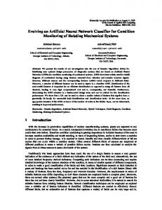
III. PWL-DFANN STRUCTURE In this section, the basic structure for the PWLDFANN is described, and its general properties are discussed. The PWL-DFANN for time series prediction is defined as a parallel connection of the L PWL neurons (PWLN) as illustrated in Fig. 1. Each PWLN performs the mathematical operations shown in Fig. 2, where the activation function is a piecewise linear Figure 2: Basic structure of the PWL neuron. (PWL) function on the interval comprising its domain. Specifically, the activation function for neuron q, is represented as (4) yq (k ) = g (vq (k )) = cTq Λ(vq (k )) , where
[
cTq = c0q
]
c1q " cσq T ,
(5)
1 ⎡ ⎤ ⎢ Λ ( v ( k )) ⎥ , 1 q ⎥ Λ (vq ) = ⎢ ⎢ ⎥ # ⎢ ⎥ Λ ( ( )) v k ⎣⎢ σ q ⎦⎥
with
(
(6)
)
⎧⎪ 1 v q ( k ) − β i + v q ( k ) − β i ; v q ≤ β σ , Λ i ( vq ( k )) = ⎨ 2 ⎪⎩ 1 2 (β σ − β i + β σ − β i ); v q > β σ
(7)
Figure 3 illustrates the contribution of each component in the definition of a general PWL function. Note that the parameters βi (i =1, ..., σ) define the partition of the PWL function (Figueroa et al., 2004). The linear combination of the inputs of PWLN q represents an M-order FIR structure, that can be written as
Figure 3: Effect of each parameter on the description of PWL function.
where the parameters to be estimated are the FIR filter bank coefficients (hq) and the parameters of the PWL functions (cq). Note that the prediction error for this structure is given by
188
J. L. FIGUEROA, J. E. COUSSEAU
L
(
)
e ( k ) = x ( k + 1) + ∑ c Tq Λ h Tq x k .
Some particular aspects observations related with this structure are the following, •
ated training algorithm, as will be discussed in the next section.
(10)
q =1
The largest improvement in the definition of the PWLN if compared with any classical neuron found in the literature, is that in our case, the nonlinearity can be adjusted for each particular application. Let us study this fact in detail. From Fig. 2 it is clear that the proposed PWLN can be thought as a linear FIR filter cascaded with a nonlinear gain. This realization characterizes the D-FANN nature of the proposed neural network. It was shown in de Figueiredo (1998a) that one can obtain a similar D-FANN as a best approximation to the Wiener model. For a recent such interpretation, see Figueroa and Cousseau (2001).
•
A complete analysis of the particular network of a single neuron, with a detailed analysis of its properties, can be found in Figueroa et al. (2004).
•
The use of PWL to represent the activation function allows the representation of any wellbehaved continuous nonlinear function. In fact, a piecewise linear function is an approximate representation of a nonlinear function. It substitutes the global nonlinear function by a series of linear sub-functions which are defined in properly partitioned sub-regions of the original nonlinear function domain. Traditionally, a general expression for this representation is given by (Lin and Unbehauen, 1990) σ f (x) = a + bT x + ∑ c j α Tj x − β j , where b and
•
Compared with preliminary studies (Figueroa et al., 2002), the PWL description in the present work includes saturation when the input signal exceeds the considered domain and allows a more selective effect of the parameters on particular regions (i.e., each entry in the vector ci involves only the function values on a portion of the domain). These two characteristics lead to improved convergence properties of the training algorithms.
•
The PWL requires the selection of the partition parameters βi for i =1, …,σ. The interval [β1,βσ] must contain the range of the signal v(k), keeping in mind that the parameters h are time varying. This is solved by choosing the interval [β1,βσ] wide enough with respect to the variation of the linear filter parameters and the input-signal range. After choosing [β1,βσ], it remains to determine the interior points. Despite that some specific application could demand for a particular (irregular) density of the interior points (Hagenblad, 1999), the common sense is to use an uniform distribution for these points. This will be the usual choice in the application examples illustrated in next sections.
•
Selection of the number of neurons L, is equivalent to the selection of the number of neurons in any traditional neural network. This is in general a non trivial task because there are no generally acceptable theories for the subject, and the solutions available in the literature are valid only for special cases. Usually, it is recommended to start with a small L, and if the fitting obtained is not fair, the number of neurons is increased. In general, a small L leads to an insufficient number of parameters to characterize the model and therefore a poor performance. On the other hand, a large L will give a good training and a bad generalization due to over fitting.
•
Another improvement of the present formulation over the preliminary studies carried out by the authors is related to the number of parameters. In Figueroa et al. (2002), the realization is formed by the linear combination of the neurons. However, in order to reduce the complexity of the realization, the linear coefficients considered there (called wi) can be modeled using the parameters of the PWL function (ci), without loss in the approximation capabilities. Note that within the space of PWL structures considered, the current method allows the best nonlinear approximation (in the least squares sense) of the desired predictor (de Figueiredo, 2000).
j =1
αj (j=1, …,σ) are M-dimensional weight vectors, a and βj (j=1, …, σ) are scalar weights. Geometrically, this function divides the input space in regions, and for each region, a linear affine model represents the system. This representation has found extensive use in the study of nonlinear circuits and systems, but can only represent nonlinearities with domain in R1 (Julián et al., 1999). Although the use of PWL descriptions is not new (Fujisawa and Kuh, 1972; Girosi et al., 1994), we choose for the PWL-DFANN a recently proposed representation that allows a very compact parameterization of the realization. We assume the PWL description as defined in Julián et al. (1999). This description is based on a simplicial partition (v=βj ,with the βj values dividing the domain in equal partitions). As a result, it is easy to verify that fixing any set of adjustable parameters (hi or ci), the approximation error is linear in the other set. These facts lead to a very low complexity realization and a simple associ-
•
IV. ALGORITHM FOR PWLN TRAINING In this section it is presented an adaptive algorithm to adjust the parameters to the time series data. To this purpose, the objective is to minimize the mean squared 189
Latin American Applied Research
38:187-193 (2008)
Table 1: Learning algorithm for the PWL-DFANN realization. ⎡⎛ L ⎞ ⎤ (11) Parameters: L = number of FIR filters E e 2 ( k ) = E ⎢⎜⎜ x ( k + 1) + ∑ c Tq Λ h Tq x k ⎟⎟ ⎥ . ⎢⎣⎝ M = order of FIR filters q =1 ⎠ ⎥⎦ σ = number of partitions adjusting the parameters hq and cq, for q = 1, …, L. µ = step-size related to h coefficients We consider the following particular updating λ = forgetting factor related to c coefficients scheme for each set of parameters. Since the error δ = initialization of P(0) signal is linear in the set of parameters cq, we proData: x posed a Recursive Least Squares (RLS) algorithm for Initialization: their estimation. On the other hand, since the prohq(0) = DCT coefficients posed realization is conceptually related to the struccq(0) = [-1 1 0 … 0]T · ture introduced in Eltoft and de Figueiredo (2000), P(0) = δ-1I where a DCT is used for the (fixed) linear part, and in For each k =1, 2, … order to maintain a low complexity realization, an For q =1, …, L.···
prediction error given by
[
]
(
)
2
stochastic gradient algorithm is proposed for the FIR coefficients hq. The design of an RLS algorithm (Haykin, 1996) for cq parameters is straightforward. To that purpose it is convenient to compile these parameters in a single matrix, C = [c1 c2 … cL], and also to define the following vector, T (12) Λ = Λ (h1T x k ) Λ (h T2 x k ) " Λ (h TL x k ) . On the other hand, the stochastic gradient algorithm used to update hq is described by ∂e ( k ) , (13) h ( k + 1) = h ( k ) − 2 μe ( k )
[
vq ( k ) = h q ( k )T x k
xˆ ( k + 1) = C T Λ e ( k ) = x ( k + 1) − xˆ ( k + 1)
For q =1, …,L h q (k + 1) = h q (k ) − 2μe(k )
]
g(k ) =
∂e(k ) ∂h q (k )
λ−1P ( k − 1) Λ 1 + λ−1 Λ T P ( k − 1) Λ
C(k +1) = C(k)+ g(k)e(k) P(k)= λ-1P(k-1)-λ-1g(k)ΛT P(k-1)
An important aspect for this updating algorithm, and for any nonlinear adaptive filter, is the selection of where µ is the step-size. In our description, the gradithe initial condition for the parameters. In particular, ent can be computed as considering the same parameters for all FIR filters hq, ∂e ( k ) ⎛⎜ T ∂Λ ( v q ) ⎞⎟ k , (14) this will move to a ill-conditioned problem. To avoid x = cq ∂h q ( k ) ⎜⎝ ∂vq ⎟⎠ this, a good choice for the initial condition of these where, if [.]j represents the j-th vector component, parameters is the DCT basis proposed in Eltoft and de Figueiredo (2000). In addition to avoid the illand conditioned problem, this selection can take profit of ⎡ ∂Λ (v q ) ⎤ , (15) the orthogonality properties of these filters. ⎥ =0 ⎢ ⎢⎣ ∂vq ⎥⎦ 1 In the next section, the proposed PWL-DFANN scheme is applied in the context of speech prediction ⎧⎪ 1 (1 + sign (vq (k ) − β j )); vq ≤ βσ . ⎡ ∂Λ (vq ) ⎤ (16) ⎢ ⎥ =⎨ 2 and illustrative practical results are discussed. . ∂v 0 ;v > β q
⎣⎢
q
q
⎦⎥ j +1
∂h q ( k )
⎪⎩
σ
q
Regarding a suitable definition of PWL gradient at the partition edges, the gradient at the partitions boundaries is defined as zero to avoid any numerical inconsistency. In Eq. 16 it is used that sign(0)=-1. The complete learning algorithm for the PWLDFANN realization is presented in Table 1. In order to guarantee convergence of the coefficients in the mean, the step-size of the LMS algorithm must be chosen as a small positive number that satisfy (Figueroa et al., 2004). ⎛ 0 < μ < min ⎜ q ⎜ ⎝
V. SIMULATION EXAMPLES Speech signals are an important class of signals that, on a short time period (5-100 ms), have statistical properties that are slowly varying. On the other hand, over longer periods of time (of the order of 1/5 s) they are highly dynamical and non-stationary. To illustrate the performance of the proposed realization, we present in this section examples of the use of PWLDFANN realization for time series prediction speech signals.
⎞, ⎟
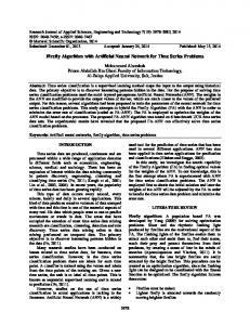
(17) A. Speech signals In this section we will apply the PWL-DFANN realization for time series prediction to predict the next samwhere ρ represents the maximum eigenvalue of maple of the speech signal depicted in Fig. 4. The rek T k trix E[(x ) x ]. Note that this expression is a simple corded time series is made up of 10000 samples, sambound for µ since ρ depends on the data and, in genpled at 8 kHz. This is the same sample signal studied in eral, it is easy to obtain a reasonable upper bound for Haykin and Li (1995) and in Eltoft and de Figueiredo σ +1 q 2 (2000), and is selected for specific comparison pur∑i=2 (ci ) . poses. The input signal segment was projected on to 12 |
2 σ +1 ρ ∑ i = 2 (c iq ) ⎟⎠
190
J. L. FIGUEROA, J. E. COUSSEAU
filters of 12-order (Eltoft and de Figueiredo, 2000)) (L = 12, M = 12). The activation function was approximated using a partition of 10 sectors, to allow a smooth approximation (σ = 10). Looking for fast convergence, the step-size of the LMS algorithm is set equal to µ =0.02, the forgetting factor of the RLS algorithm is set equal to λ =0.998 (similar to the value used in Eltoft and de Figueiredo, 2000), and the initial correlation matrix coefficient is fixed as δ=50. The squared prediction error is depicted in Fig. 5. For quantitative comparison with other prediction algorithms, we used the following performance index introduced by Haykin and Li (1995),
As can be concluded from this, and other exhaustive computer simulations, the index performance obtained for the PWL-DFANN is highly competitive if compared with the other approaches. Table 2 includes also the number of parameters to be updated in each implementation1. An important aspect to consider is the benefit of the adaptation of parameters h. Note that the DFANN (Eltoft and de Figueiredo, 2000) uses a fixed set of parameters. When we consider these parameters fixed at the initial condition, the performance obtained is given by Rp = 27.81. This value is slightly lower than the performance obtained when these parameters are adjusted. As a consequence, maintain fixed h pak rameters is an interesting alternative, mostly because 2 ⎛δ ⎞ (18) the set of parameters to be adjusted is reduced to 132. R p = 10 log 10 ⎜ s2 ⎟ , ⎜δ ⎟ ⎝ p⎠ As mentioned above, the initial values of h are set as 2 where δ s is the mean square value of the incoming the DCT basis (Eltoft and de Figueiredo, 2000). Figure 6 illustrates the dependence of Rp with the signal, and δ p2 is the corresponding value of the prenumber of neurons L. It can be observed with this figdiction error. ure that with an increase of L leads to an improvement Comparison results using previous index are sum- in the index performance Rp. However, use of large L marized in Table 2, where other values found in the (higher than 12 for this example) leads in general to literature are also included for this example. Nomi- produce over-fitting. Figure 7 illustrates the dependnally, a linear adaptive predictor (LAP), a pipeline ence of performance index Rp with the step-size µ. recurrent neural network (PRNN; Haykin and Li, From this figure it is clear that, for reasonable values 1995), a multilayer perceptron (MP) and the DFANN of the step size µ, the adaptation of h allows a small (Eltoft and de Figueiredo, 2000). improvement of the performance index. Finally, a study of the dependence on the estimation of C of the RLS forgetting factor λ is illustrated in Fig. 8. In this plot the values of Rp are depicted for several values of λ. As can be concluded, the selection of λ is not critical to obtain a good performance using the PWL-DFANN. B. Handel’s Hallelujah Chorus In this example a set of 72000 samples, extracted from the Handel’s Hallelujah Chorus, is used for quantitative comparison. The prediction algorithms used in the comparison are: a linear adaptive predictor (LAP), the pipeline recurrent neural network (PRNN; Haykin and Li, 1995), the D-FANN (Eltoft and de Figueiredo, 2000) and the proposed PWLDFANN. Comparison results, using previous performance index, are summaFigure 4: Speech signal and prediction obtained using rized in Table 3. PWL-DFANN.
Table 2: Comparative results for different non linear predictors in Example 1. Technique Parameters Rp PWL-DFANN 27.8945 276 DCT-DFANN 27.55 36 (†) 27.2869 288 PWL-DFANN(‡) PRNN 25.14 52 LAP 22.01 12 MP ≈ 18 169(*) †
‡
( ) Plus 144 fixed coefficients taken as DCT.; ( ) Figueroa et al. * (2002); ( ) MP with 12 neurons on the hidden layer 1
Figure 5: Squared prediction error using PWL-DFANN realization.
The results used for comparison purposes are taken from the literatura (Eltoft and de Figueiredo, 2000; Figueroa et al., 2002; Haykin and Li, 1995).
191
Latin American Applied Research
Figure 6: Dependence of Rp as function of the number of neurons L.
Figure 7: Dependence of Rp as function of the step-size µ. Table 3: Comparative results for different non linear predictors in Example 2. Technique Rp PWL-DFANN 18.0771 DCT-DFANN 17.0065 PRNN 16.0899 LAP 15.0008
From this data the values of the performance index obtained for the PWL-DFANN shows to be high-ly competitive if compared with the other approaches.
Figure 8: Dependence of Rp as function of the forgetting factor λ for the RLS-algorithm.
38:187-193 (2008)
VI. CONCLUSIONS In this paper, we have used a PWL-DFANN to build a nonlinear, adaptive time series predictor. The compact PWL description utilized for the PWL-DFANN includes saturation when the input signal exceeds the considered domain. This particular definition allows a selective effect of the parameters on particular regions. Training is a combination of a stochastic gradient algorithm and a RLS algorithm, leading to robust experimental results. The resulting realization is simple and the performance shows that this structure can be successfully used to perform prediction of highly nonstationary and dynamic speech signals. REFERENCES Chen, S., C.F.N. Cowan and P.M. Grant, “Orthogonal least squares learning algorithm for radial basis function networks”, IEEE Trans. Neural Networks, 2, 302-309 (1991). de Figueiredo, R.J.P. and T.A. Dwyer, “A best approximation framework and implementation for simulation of large-scale nonlinear systems,” IEEE Trans. Circuits Syst., CAS-27, 1005-1014 (1980). de Figueiredo, R.J.P., “A generalized Fock space framework for nonlinear system and signal analysis”, IEEE Trans. Circuits Syst., CAS-30, 637-647 (1983). de Figueiredo, R.J.P., “A neural network model for nonlinear predictive coding in Fock space,” IEEE Int. Symp. Circuits and Systems, Chicago, IL, 21642167 (1993). de Figueiredo, R.J.P., “Optimal interpolating and smoothing functional artificial neural networks (FANNs) based on a generalized Fock space framework,” Circuits, Systems, and Signal Processing, 17, 271-87 (1998a). de Figueiredo, R.J.P., “Beyond Volterra and Wiener: Some new results and open problems in nonlinear signal and image processing,” Midwest Symposium on Circuits and Systems, , 124-127 (1998b). de Figueiredo, R.J.P., “A reproducing kernel Hilbert space (RKHS) approach to the optimal modeling, identification, and design of nonlinear adaptive systems,” IEEE Symp. on Adaptive Systems for Signal Processing, Comm. and Control, 42-47 (2000). Eltoft, T. and R.J.P. de Figueiredo, “A DCT-Based DFANN for nonlinear adaptive time series prediction,” IEEE Trans. Circuits Syst., Part II, 47, 11311134 (2000). Figueroa, J.L. and J.E. Cousseau, “A Wiener CPWL Adaptive Filter,” 2nd. IEEE South-American Workshop on Circuits and Systems, SAWCAS’2001, Buenos Aires, Argentina, 2001. Figueroa, J.L., J.E. Cousseau and R.J.P. de Figueiredo, “A Piecewise Linear Dynamical Functional Artificial Neural Network (PWL-DFANN) for Nonlinear Adaptive Time Series Prediction,” IEEE Int. Symp. Circuits and Systems, I29-I32 (2002). 192
J. L. FIGUEROA, J. E. COUSSEAU
Figueroa, J.L., J.E. Cousseau and R.J.P. de Figueiredo, “A low complexity simplicial canonical piece-wise linear adaptive filter,” Circ., Syst. and Signal Proc. Journal, 23, 365-386 (2004). Fujisawa, T. and E.S. Kuh, “Piecewise-linear theory of nonlinear networks,” SIAM J. Appl. Math., 22, 307-328 (1972). Girosi, F., M. Jones and T. Poggio, “Regularization theory and neural networks architecture,” Neural Computation, 7, 219-269 (1995). Hagenblad, A., “Aspects of the identification of Wiener models,” M.Sc thesis dissertation, Linkoping University, Sweden (1999). Haykin, S., Adaptive Filter Theory, Prentice Hall, N.J. (1996). Haykin, S. and L. Li, “Nonlinear adaptive prediction of nonstacionary signals,” IEEE Trans. Signal Processing, 43, 526-535 (1995). Julián, P., A. Desages and O. Agamennoni, “High Level Canonical Piecewise Linear Representation Using a Simplicial Partition,” IEEE Trans. Circuits Syst., Part I, 46, 463-480 (1999). Knecht, K.G., “Nonlinear noise filtering and beamforming using the perceptron and its Volterra approximation,” IEEE Trans. Acoust. Speech Signal Processing, 2, 55-62 (1994).
Lendasse, A., E. Oja, O. Simula, and M. Verleysen, “Times series prediction competition: The CATS benchmarck,” Neurocomputing, 70, 2325-2329 (2007). Lin, J.N. and R. Unbehauen, “Adaptive nonlinear digital filter with canonical piecewise linear structure,” IEEE Trans. Circuits Syst., CAS-37, 347-353 (1990). Newcomb, R.W. and R.J.P. de Figueiredo, “A multiinput multi-output functional artificial neural network,” J. of Intelligent and Fuzzy systems, 4, 207213 (1996). Schetzen, M., “Nonlinear system modeling based on the Wiener theory,” Proc. IEEE, 69, 1557-1573 (1981). Shuzo, S. and K. Nakata, Fundamentals of Speech Signal Processing, Academic Press, New York (1985) Weigend, A., B. Huberman and D. Rumelhart, “Predicting the future: A connectionist approach,” Int. J. Neural Syst., 7, 403-430 (1990). Werbos, P., “Generalization of backpropagation with application to a recurrent gas market model,” Neural Networks, 1, 339-365 (1988). Zyla, L.V. and R.J.P. de Figueiredo, “Nonlinear system identification based on a Fock space framework,” SIAM J. Contr. Optimiz., 31, 931-939 (1993)
Received: November 22, 2006. Accepted: October 12, 2007. Recommended by Subject Editor: Julio Braslavsky 193