Oct 8, 2002 - Solid state realizations are also under way in several ex- perimental ...... [10] S. Fishman, D.R. Grempel, and R.E. Prange, Phys. Rev. Lett.
Dynamical localization simulated on a few qubits quantum computer Giuliano Benenti(a) , Giulio Casati(a,b) , Simone Montangero(a), and Dima L. Shepelyansky(c) (a)
arXiv:quant-ph/0210052v1 8 Oct 2002
International Center for the Study of Dynamical Systems, Universit` a degli Studi dell’Insubria and Istituto Nazionale per la Fisica della Materia, Unit` a di Como, Via Valleggio 11, 22100 Como, Italy (b) Istituto Nazionale di Fisica Nucleare, Sezione di Milano, Via Celoria 16, 20133 Milano, Italy (c) Laboratoire de Physique Quantique, UMR 5626 du CNRS, Universit´e Paul Sabatier, 31062 Toulouse Cedex 4, France (October 8, 2002) We show that a quantum computer operating with a small number of qubits can simulate the dynamical localization of classical chaos in a system described by the quantum sawtooth map model. The dynamics of the system is computed efficiently up to a time t ≥ ℓ, and then the localization length ℓ can be obtained with accuracy ν by means of order 1/ν 2 computer runs, followed by coarse grained projective measurements on the computational basis. We also show that in the presence of static imperfections a reliable computation of the localization length is possible without error correction up to an imperfection threshold which drops polynomially with the number of qubits. PACS numbers: 03.67.Lx, 05.45.Mt, 24.10.Cn
cal chaos. Dynamical localization is one of the most interesting phenomena that characterize the quantum behavior of classically chaotic systems: Quantum interference effects suppress chaotic diffusion in momentum, leading to exponentially localized wave functions. This phenomenon was first found and studied in the quantum kicked rotator model [9] and has profound analogies with Anderson localization of electronic transport in disordered materials [10]. Dynamical localization has been observed experimentally in the microwave ionization of Rydberg atoms [11] and is now actively studied in experiments with cold atoms [12]. In this paper, we study dynamical localization for the quantum sawtooth map, using the algorithm developed in Ref. [13]. This algorithm has some specific advantages with respect to similar algorithms for the simulation of other dynamical systems, for instance the kicked rotator [14]. There are no extra work space qubits, namely all the qubits are used to simulate the dynamics of the system. This implies that less than 40 qubits would be sufficient to make simulations inaccessible to present day supercomputers. We note that this figure has to be compared with the more than 1000 qubits required to the Shor’s algorithm to outperform classical computations. We will also show that in this model dynamical localization could be observed already with 6 qubits. The paper is organized as follows. In Section II we describe the sawtooth map model, focusing on the regime of dynamical localization. In Section III we show that a quantum computer operating with few qubits can indeed perform simulations of dynamical localization. In Section IV we discuss how to extract information (the localization length) from the quantum computer wave function. In Section V we study the stability of those computations in the presence of static imperfections in the quantum computer hardware. In Section VI we discuss the transition to quantum chaos, induced by static imperfections, in the quasienergy spectral statistics. In
I. INTRODUCTION
Recent experimental progress in nuclear magnetic resonance (NMR)-based quantum processors allowed the demonstration of quantum algorithms [1], including Grover’s algorithm [2] and quantum Fourier transform [3]. More recently, it has been possible to implement the simplest instance of Shor’s algorithm, namely the factorization of 15, using 7 qubits and a sequence of about 300 spin-selective radio-frequency pulses [4]. In parallel, thanks to the development of techniques for the manipulation of cold atoms in linear traps, the realization of up to 50 two-qubit control-not gates within the relevant decoherence time scale is currently becoming possible [5]. Solid state realizations are also under way in several experimental groups working with various solid state devices. In particular, it has been demonstrated that a superconducting tunnel junction circuit can behave as an artificial spin 1/2 atom, whose evolution can be controlled by applying microwave pulses. The quality factor of quantum coherence is sufficiently high to envisage the realization of two-qubit gates based on capacitively coupled circuits of this type [6]. In this context, it is of primary importance to find efficient quantum algorithms, that could be usefully simulated with a small number of qubits. Such algorithms would naturally become the ideal software for demonstrative experiments in the coming generation of quantum processors. Dynamical models represent a natural testing ground for quantum information processors. The algorithm for the quantum baker’s map [7] has been recently implemented on a three qubit NMR quantum processor [8]. These experiments tested the sensitivity to perturbations, in a system which is characterized by chaotic unpredictable dynamics in the classical limit. In this paper we show that quantum computers can simulate efficiently the quantum localization of classi1
t⋆ ≈ Dn ≈ (π 2 /3)k 2 ,
Section VII we present our conclusions.
where Dn is the classical diffusion coefficient, measured in number of levels (< (∆n)2 >≈ Dn t). For t > t⋆ only ∆n ∼ Dn levels are populated and the localization length ℓ ∼ ∆n for the average probability distribution is approximately equal [17]:
II. THE MODEL
The quantum sawtooth map is the quantized version of the classical sawtooth map, which is given by n = n + k(θ − π),
θ = θ + T n,
(1)
ℓ ≈ Dn
where (n, θ) are conjugated action-angle variables (0 ≤ θ < 2π), and the over bars denote the variables after one map iteration. Introducing the rescaled momentum variable p = T n, one can see that the classical dynamics depends only on the single parameter K = kT . The map (1) can be studied on the cylinder (p ∈ (−∞, +∞)), which can also be closed to form a torus of length 2πL, where L is an integer. For K > 0, the motion is completely chaotic and exhibits normal diffusion: < (∆p)2 >≈ D(K)t, where t is the discrete time measured in units of map iterations and the average < · · · > is performed over an ensemble of particles with initial momentum p0 and random phases 0 ≤ θ < 2π. For K > 1 the diffusion coefficient is well approximated by the random phase approximation, D(K) ≈ (π 2 /3)K 2 . The quantum evolution in one map iteration is deˆ (called Floquet operator) scribed by a unitary operator U acting on the wave function ψ: 2 ˆ /2 ˆ ψ = e−iT nˆ 2 /2 eik(θ−π) ψ=U ψ,
(3)
(4)
Thus the quantum localization can be detected if ℓ is smaller than the system size N . √ In the√following we consider K = 2, two values of k, k = 3 and k = 2, and 6 ≤ nq ≤ √ 21, so that the above analytical estimate gives ℓ(k = 3) ≈ 10 and ℓ(k = 2) ≈ 13 < N . We assume that at t = 0 the system ˆ is in a momentum eigenstate, ψ(n) = δnn0 . Since this is a quantum register state, it can be obtained in O(nq ) onequbit operations starting from the fiducial state (“ground state”) n of the quantum computer hardware.
III. SIMULATION OF DYNAMICAL LOCALIZATION
An exponentially efficient quantum algorithm for the simulation of the map (2) was described in Refs. [13,16]. It is based on the forward/backward quantum Fourier transform [1] between momentum and coordinate bases: On the whole, it requires ng = 3n2q + nq gates per map iteration (3n2q − nq controlled-phase shifts and 2nq Hadamard gates). This number has to be compared with the O(N log N ) operations required to a classical computer to simulate one map iteration by means of the fast Fourier transform. In Fig. 1, we show that, using our quantum algorithm, exponential localization can be clearly seen already with nq = 6 qubits. After the break time t⋆ , the probability distribution over the momentum eigenbasis decays exponentially,
(2)
where n ˆ = −i∂/∂θ and ψ(θ + 2π) = ψ(θ) (we set ¯h = 1). The classical limit corresponds to k → ∞, T → 0, and K = kT = const. In Refs. [13,15,16] we studied the map (2) in the semiclassical regime. This is possible by increasing the number of qubits nq = log2 N (N is the total number of levels), with T = 2πL/N , K = const. In this way, the number of levels inside the “unit cell” −π ≤ p < π (L = 1) grows exponentially with the number of qubits (−N/2 ≤ n < N/2), and the effective Planck constant h ¯ eff ∼ ¯ h/k ∼ 1/N → 0 when N → ∞. Differently from previous studies, in this paper we study the map (2) in the deep quantum regime of dynamical localization. For this purpose, we keep k, K constant. Thus the effective Planck constant is fixed and the number of cells L grows exponentially with the number of qubits (L = T N/2π). In this case, one studies the quantum sawtooth map on the cylinder (n ∈ (−∞, +∞)), which is cut-off to a finite number of cells due to the finite quantum (or classical) computer memory. We stress again that, since in a quantum computer the memory capabilities grow exponentially with the number of qubits, already with less than 40 qubits one could make simulations of systems inaccessible for today’s supercomputers. Similar to other models of quantum chaos [9], the quantum interference in the sawtooth map leads to suppression of classical chaotic diffusion after a break time
� � 1 2|n − n0 | 2 ˆ , Wn = |ψ(n)| ≈ exp − ℓ ℓ
(5)
with n0 = 0 the initial momentum value. Here the localization length is ℓ ≈ 12, and classical diffusion is suppressed after a break time t⋆ ≈ ℓ, in agreement with the estimates (3)-(4). This requires a number Ng ≈ 3n2q ℓ ∼ 103 of one- or two-qubit quantum gates. The full curve of Fig. 1 shows that an exponentially localized distribution indeed appears at t ≈ t⋆ . Such a distribution is frozen in time, apart from quantum fluctuations, which we partially smooth out by averaging over a few map steps. The localization can be seen by the comparison of the probability distributions taken immediately after t⋆ (full curve 2
in Fig. 1) and at a much larger time t = 300 ≈ 25t⋆ (dashed curve in the same figure).
IV. MEASUREMENTS
We also note that the asymptotic tails of the wave functions decay as a power law(see Fig. 2),
We now discuss how it would be possible to extract information (the value of the localization length) from a quantum computer simulating the above described dynamics. The localization length can be measured by running the algorithm several times up to a time t > t⋆ . Each run is followed by a standard projective measurement on the computational (momentum) basis. The outcomes of the measurements can be stored in histogram bins of width δn ∝ ℓ, and then the localization length can be extracted from a fit of the exponential decay of this coarse-grained distribution over the momentum basis. In this way the localization length can be obtained with accuracy ν after the order of 1/ν 2 computer runs. It is important to note that it is sufficient to perform a coarse grained measurement to generate a coarse grained distribution. This means that it will be sufficient to measure the most significant qubits, and ignore those that would give a measurement accuracy below the coarse graining δn. Thus, the number of runs and measurements is independent of ℓ. However, it is necessary to make about t⋆ ∼ ℓ map iterations to obtain the localized distribution (see Eqs. (3,4)). This is true both for the present quantum algorithm and for classical computation. This implies that a classical computer needs O(ℓ2 log ℓ) operations to extract the localization length, while a quantum computer would require O(ℓ(log ℓ)2 ) elementary gates (classically one can use a basis size N ∼ ℓ to detect localization). In this sense, for ℓ ∼ N = 2nq the quantum computer gives a square root speed up if both classical and quantum computers perform O(N ) map iterations. However, for a fixed number of iterations t the quantum computation gives an exponential gain. For ℓ ≪ N such a gain can be very important for more complex physical models, in order to check if the system is truly localized [20].
Wn ∝
1 . |n − n0 |4
(6)
This happens due to the discontinuity in the kicking force of Eq. (1), f (θ) = k(θ − π), when the angle variable θ = 0. For that reason the matrix elements of the ˆ for the quantum map one period evolution operator U (2) decay as a power law in the momentum eigenbasis: ˆ |mi ∼ 1/|n − m|α , with α = 2. This case Unm = hn|U was investigated for random matrices, where it was shown that eigenfunctions are also algebraically localized with the same exponent α [18]. We also note that dynamical localization in discontinuous systems was studied in [19]. Since the localization picture is not very sensitive to the behavior of the tails of the wave function, a rough estimate of the crossover between the exponential decay (5) and the power law decay (6) is given by their crossing point, nc ∼
3 ℓ log ℓ, 2
Wn (nc ) ∼
1 . ℓ4 log ℓ
(7)
This implies that by increasing ℓ the exponential localization is pushed to larger momentum windows and down to smaller probabilities.
log Wn
−1
−2
V. EFFECTS OF STATIC IMPERFECTIONS
In order to study the effects of static imperfections on the stability of the above described algorithm, we model the quantum computer hardware as a linear array of qubits with static imperfections, represented by fluctuations in the individual qubit energies and residual short-range inter-qubit couplings [21]. The model is described by the following many-body Hamiltonian: X X ˆs = Jij σ ˆix σ ˆjx , (8) (∆0 + δi )ˆ σiz + H
−3
−4 −30
−20
−10
0
10
20
30
n FIG. 1. Exact quantum computation of probability distribution √ over the momentum basis with nq = 6 qubits for k = 3 and initial momentum n0 = 0; the average is taken in the intervals 10 ≤ t ≤ 20 (full curve) and 290 ≤ t ≤ 300 (dashed curve). The straight line fit, Wn ∝ exp(−2|n|/ℓ), gives a localization length ℓ ≈ 12. Here and in the following figures, the logarithms are decimal.
i
i≈ Dn (ǫ)t.
This is an important characteristic related to transport properties of the system; (ii) the inverse participation ratio
(9)
where ˆ g (τ ) = H
X k
ˆk. δ(τ − kτg )h
(10)
ξ=P
ˆ k realizes the k-th elementary gate according to Here h the sequence prescribed by the algorithm. We assume that the phase accumulation given by ∆0 is eliminated by standard spin echo techniques [1]. In this case, the remaining terms in the static Hamiltonian (8) can be seen as residual terms after imperfect spin echoes and give unwanted phase rotations and qubit couplings. The effect of static imperfections on the probability distribution over the momentum basis is shown in Fig. 2, for k = 2, nq = 11, t = 100, J = 0, and different rescaled imperfection strengths ǫ = δτg . For ǫ = 10−4 , the localization peak is reproduced with high fidelity, while the tails of the wave function are strongly enhanced. This is due to the fact that errors affecting the most significant qubits can induce a direct transfer of probability very far in the momentum basis [22,13]. For ǫ = 10−3 a measurement of the decay of the localization peak would overestimate the localization length by a factor two, while for ǫ = 10−2 any trace of dynamical localization has been destroyed.
2
600
400
200
0
0
5
10
15
20
t FIG. 3. Dependence of the wave function second moment on time, for k = 2, nq = 11, J = 0 (full symbols) and J = δ (empty symbols) at ǫ = 0 (circles), 5 × 10⁻⁵ (squares), 10−4 (diamonds), and 2 × 10⁻⁴ (triangles). The straight lines fits give the diffusion coefficient Dn (ǫ). The curves are averaged over 10 disorder realizations and 10 initial conditions n0 ∈ [−5, 5[.
2 0
log Wn
(12)
800
4
−2 −4 −6 −8
In Fig. 3 we show < (∆n)2 > as a function of time, for nq = 11 qubits, J = 0, and different imperfection strengths ǫ. By means of these curves we extract the diffusion coefficients Dn (ǫ) from linear fits extended to the first few map steps. In the same figure, we show that similar curves are obtained for J = δ. The dependence of the inverse participation ratio on t is shown in Fig. 4, again for k = 2, nq = 11. We note that, for imperfection strengths strong enough to induce huge variations in the diffusion coefficient (Dn (ǫ) ≫ Dn (0)),
−10 −1000
1 ; 2 n Wn
this quantity determines the number of basis states significantly populated by the wave function and gives an estimate of the localization length of the system. We stress that, differently from the previous quantity, ξ is local in the localized regime, i.e. it is insensitive to the behavior of exponentially small tails.
6
−12
(11)
−500
0
500
1000
n FIG. 2. Probability distributions for k = 2, nq = 11, n0 = 0, J = 0. From bottom to top: ǫ = 0, 10−4 (gray line), 10−3 (shifted up by a factor 4), and 10−2 (shifted up by a factor 8). The straight line gives a localization length ℓ ≈ 15.
4
in good agreement with the data of Fig. 7.
ξ is only slightly modified (ξ(ǫ) ≈ ξ(0)). Iterating the map (2) long enough (t > ξ(ǫ)), we get the saturation value ξ∞ (ǫ). This quantity increases with ǫ and one has complete delocalization when ξ∞ (ǫ) ∼ N (this is evident for ǫ = 5 × 10− 3 in Fig. 4; in this case ξ saturates after t < 100 map iterations). Again we note that similar curves are obtained for J = δ (see Fig. 4).
10
log Dn
8
1000
6
4
800
ξ
2 600
0
400 200 0
0
50
100
150
200
FIG. 4. Time dependence of the inverse participation ratio ξ for k = 2, nq = 11 qubits, J = 0 (solid lines) and J = δ (dashed lines). From bottom to top: ǫ = 0, 5 × 10⁻⁴ , 10−3 , 2 × 10⁻³ , 5 × 10⁻³ . The curves are averaged as in Fig. 3.
In Fig. 5 we plot the dependence of diffusion coefficient Dn on ǫ for different nq values. From each curve we extract the critical imperfection strength ǫD (nq ) corresponding to doubling of the diffusion coefficient, Dn (ǫD ) = 2Dn (0). The data of Fig. 7 show that ǫD drops exponentially with nq . This result is similar to the one found in [22] for noisy gate errors and can be explained by means of the following argument. Static imperfections can couple states very far in momentum space via a single spin flip. As a consequence, they create nq peaks [22] with probability Wp ∼ ǫ2eff t in each peak. Here ǫeff ∼ δn2q τg = ǫn2q is the effective perturbation strength, with n2q τg time between Hadamard gates acting on a given qubit. These gates transfer the accumulated phase error ǫeff into amplitude errors. Integrating the contribution of each peak, one gets (13)
Dǫ ∼ ǫ2 n4q N 2 .
(14)
−6
−5
−4
log ε
−3
−2
−1
FIG. 5. Dependence of the diffusion coefficient Dn on the imperfection strength ǫ for k = 2, J = 0 (full symbols), nq = 6 (triangles down), 8 (stars), 10 (triangles up), 12 (squares), 15 (diamonds), 18 (circles), and for J = δ, nq = 10 (empty triangles). The straight lines show the theoretical dependence D ∝ ǫ2 (full line, see Eq. (14)) and the result without imperfections, D(ǫ = 0) ≈ 16 (chain line).
t
< (∆n)2 >∼ Wp N 2 ∼ Dǫ t,
−7
4
log ξ∞
3
2
1
−4
−3
log ε
−2
−1
FIG. 6. Dependence of the saturation value ξ∞ of the inverse participation ratio on the imperfection strength ǫ, with same parameter values and same meaning of symbols as in the previous figure. The straight line shows the result without imperfections, ξ∞ (ǫ = 0) ≈ 14.
with
In Fig. 6 we show the dependence of the inverse participation ratio ξ(ǫ) on ǫ for different number of qubits nq . From each curve we extract two critical imperfection strengths: (i) ǫξE , to get an inverse participation ratio equal to a given fraction of the full Hilbert space, for example ξ = N/4. This threshold is significant of the transition
One can estimate the critical value ǫD to double the exact (ǫ = 0) diffusion coefficient from Dǫ = Dn (ǫ = 0), giving p Dn (0) , (15) ǫD ∼ n2q N 5
to ergodic completely delocalized wave functions. (ii) ǫξ , to double the exact inverse participation ratio. We stress that this quantity gives a rough estimate of the imperfection threshold for reliable quantum computation of localization in the absence of error correction. The dependence of ǫξE and ǫξ on nq are shown in Fig. 7. These quantities drop polynomially with nq , in sharp contrast with the exponential drop of ǫD . This algebraic threshold can be understood as follows. The eigenstates ˆ in of the unperturbed (ǫ = 0, J=0) Floquet operator U (2) can be written as φ(0) α =
N X
c(m) α um ,
couplings between Floquet eigenstates. However, an estimate similar to (17), which does not modify the functional dependence (18), can be derived. We stress the striking difference between this polynomial scaling and the exponential scaling for the mixing of unperturbed eigenstates obtained in the ergodic regime (in which ℓ ∼ N ) and in the more general quasi-integrable regime [15,16]. We also note that the different sensitivity of local and non local quantities was pointed out in [22]. However, the authors of Ref. [22] considered the effect of noisy gates, while we consider internal static imperfections. −2
(16)
m=1
−3
where um are the quantum register (momentum) states. (m) In the localized regime, cα ’s are randomly fluctuating inside the localization domain of size ℓ, and exponentially small outside √ it. Wave function normalization imposes (m) |cα | ∼ 1/ ℓ. Due to exponential localization, static imperfections couple significantly the unperturbed eigenfunctions only when their localization domains overlap. We estimate in this case the transition matrix elements according to perturbation theory. For J = 0, they have a typical value Vtyp ∼
∼
(0) |hφβ |
nq X
(m)⋆ (m)
c(m) α cβ
η
m=1
log ε
−7 −8 6
ℓ X
ℓ X
(17)
12
14
16
18
20
VI. SPECTRAL STATISTICS
In this Section, we show that spectral statistics is an ideally suited tool to detect the destruction of localization by static imperfections. We study the spectral statistics of the Floquet operator for a quantum computer running the quantum sawtooth map algorithm in the presence of static imperfections, � � Z τg ng ˆ ) , ˆǫ = exp −i dτ H(τ (20) U 0
where H(τ ) is the Hamiltonian (9) and ng the number of gates per map iteration. We construct numerically the Floquet operator in the computational (momentum) basis, using the fact that a single map iteration of each quantum register state gives a column in the matrix representation of this operator. Then we diagonalize the Floquet matrix and get the so-called quasienergy eigen(ǫ) (ǫ) values λα and eigenvectors φα ,
The analytical result 1
10
FIG. 7. Dependence of the critical imperfection strengths on the number of qubits for k = 2, J = 0: thresholds ǫD (circles), ǫξE (full diamonds), and ǫξ (empty diamonds). The full line gives the theoretical dependence −5/2 , withpthe fitting constant A ≈ 0.5. The dashed ǫξE = Anq lines gives ǫD = B D(ǫ = 0)2−nq n−2 q , with the fitting constant B ≈ 3.6.
−1/2 . | ∼ ǫn5/2 q ℓ
5/2 √ nq ℓ
8
nq
√ In this expression, the typical phase error is δ nq η (m) (sum of nq random detunings δi ’s), with η (m) random sign, and τg ng ∼ τg n2q is the time used by the quantum computer to simulate one map step. The last estimate in (17) results from the sum of order ℓ terms of amplitude (m) (m)⋆ |cα cβ | ∼ 1/ℓ and random phases. Since the spacing between significantly coupled quasi-energy eigenstates is ∆E ∼ 1/ℓ, the threshold for the breaking of perturbation theory can be estimated as √ ℓ ∼ 1. (18) Vtyp /∆E ∼ ǫξE n5/2 q
ǫξE ∼
−5 −6
δi σ ˆiz τg ng |φ(0) α i|
i=1 nq X (n)⋆ δi hun |ˆ σiz |um i| τg n2q | c(m) c α β m,n=1 i=1
∼ ǫn5/2 q |
−4
(19)
is confirmed by the numerical data of Fig. 7. For the case J = δ, the threshold ǫξE is reduced (see Fig. 4) since residual inter-qubit interactions introduce further 6
ˆǫ φ(ǫ) = exp(iλ(ǫ) )φ(ǫ) . U α α α
(21)
VII. CONCLUSIONS
A convenient way to characterize the spectral properties of the system is to study the level spacing statistics P (s), where P (s)ds gives the probability to find two adjacent levels (quasienergies) whose energy difference, normalized to the average level spacing, belongs to the interval [s, s+ ds] (see e.g. [23,24]). In the localized regime, Floquet eigenvectors with very close eigenvalues may lay so far apart that their overlap is negligible. As a consequence, eigenvalues are uncorrelated, that is their spectral statistic is given by the Poisson distribution, PP (s) = exp(−s).
In summary, we have shown that a quantum computer operating with a small number of qubits can simulate efficiently quantum localization effects. The evaluation of the localization length ℓ with accuracy ν requires a number of computer runs of order 1/ν 2 , followed by a projective measurement in the computational (momentum) basis. We stress that, in the presence of static imperfections, a reliable computation of the localization length is possible even without quantum error correction, up to an imperfection strength threshold which drops only algebraically with the number of qubits. We also stress that localization is a purely quantum phenomenon, which is quite fragile in the presence of noise [25,22]. Therefore we believe that the simulation of the physics of localization can be an interesting testing ground for the coming generation of quantum processors operating in the presence of decoherence and static imperfections.
(22)
On the contrary, in the delocalized regime wave functions are ergodic, and their overlap gives a significant coupling matrix element between states nearby in energy. In this case the spectral statistics P (s) follows the Wigner-Dyson distribution, � � 4s2 32s2 , (23) PW D (s) = 2 exp − π π typical of random matrices in the absence of time reversal symmetry [23,24] (static imperfections break this symmetry). In Fig. 8 we show that static imperfections indeed induce a crossover from the localized regime with the Poisson statistics to quantum chaos characterized by Wigner-Dyson statistics. We have also studied this crossover as a function of the number of qubits (data not shown): the threshold ǫc (nq ) for the emergence of quan−5/2 tum chaos is consistent with the scaling ǫc (nq ) ∝ nq , in agreement with the threshold (19) obtained for the mixing of unperturbed eigenfunctions.
This research was supported in part by the EC RTN contract HPRN-CT-2000-0156, the NSA and ARDA under ARO contracts No. DAAD19-01-1-0553 and No. DAAD19-02-1-0086, the project EDIQIP of the IST-FET programme of the EC and the PRIN-2000 “Chaos and localization in classical and quantum mechanics”.
[1] See, e.g., M.A. Nielsen and I.L. Chuang, Quantum Computation and Quantum Information (Cambridge University Press, Cambridge, 2000). [2] L.M.K. Vandersypen, M. Steffen, M.H. Sherwood, C.S. Yannoni, G. Breyta, and I.L. Chuang, Appl. Phys. Lett. 76, 646 (2000). [3] Y.S. Weinstein, M.A. Pravia, E.M. Fortunato, S. Lloyd, and D.G. Cory, Phys. Rev. Lett. 86, 1889 (2001). [4] L.M.K. Vandersypen, M. Steffen, G. Breyta, C.S. Yannoni, M.H. Sherwood and I.L. Chuang, Nature 414, 883 (2001). [5] D. Leibfried, C. Roos, P. Barton, H. Rohde, S. Gulde, A.B. Muindt, G. Reymond, M. Lederbauer, F. SchmidtKaler, J. Eschner, and R. Blatt, in Atomic Physics 17, Proceedings of the XVII International Conference on Atomic Physics, edited by E. Arimondo, P. De Natale, and M. Inguscio (AIP, New York, 2001), quantph/0009105. [6] D. Vion, A. Aassime, A. Cottet, P. Joyez, H. Pothier, C. Urbina, D. Esteve, and M.H. Devoret, Science 296, 886 (2002). [7] R. Schack, Phys. Rev. A 57, 1634 (1998). [8] Y.S. Weinstein, S. Lloyd, J.V. Emerson, and D.G. Cory, quant-ph/0201064, Phys. Rev. Lett. (in press).
1.0
0.8
P(s)
0.6
0.4
0.2
0.0 0.0
0.5
1.0
1.5
2.0
2.5
3.0
s FIG. 8. Level spacing statistics for k = 2, nq = 11, J = 0, ǫ = 10−5 (circles) and ǫ = 2.6 × 10⁻³ (squares). The dashed and full curves give the Poisson (22) and Wigner-Dyson distribution (23), respectively. In order to reduce statistical fluctuations, data are averaged over ND = 5 random realizations of δi ’s, so that the total number of spacings is ND N ≈ 104 .
7
[17] D.L. Shepelyansky, Physica D 28, 103 (1987). [18] A.D. Mirlin, Y.V. Fyodorov, F.-M. Dittes, J. Quezada, and T.H. Seligman, Phys. Rev. E 54, 3221 (1996). [19] F. Borgonovi, G. Casati, and B. Li, Phys. Rev. Lett. 77, 4744 (1996); F. Borgonovi, Phys. Rev. Lett. 80, 4653 (1998); G. Casati and T. Prosen, Phys. Rev. E 59, R2516 (1999). [20] This is not an easy task in many-body quantum systems but also in single particle models like the kicked Harper model, see T. Prosen, I.I. Satija, and N. Shah, Phys. Rev. Lett. 87, 066601 (2001), and references therein. [21] B. Georgeot and D.L. Shepelyansky, Phys. Rev. E 62, 3504 (2000); 62, 6366 (2000); G. Benenti, G. Casati, and D.L. Shepelyansky, Eur. Phys. J. D 17, 265 (2001). [22] P.H. Song and D.L. Shepelyansky, Phys. Rev. Lett. 86, 2162 (2001). [23] O. Bohigas, in Les Houches Lecture Series, edited by M.J. Giannoni, A. Voros, and J. Zinn-Justin (North-Holland, Amsterdam, 1991), Vol. 52. [24] T. Guhr, A. M¨ uller-Groeling, and H.A. Weidenm¨ uller, Phys. Rep. 299, 189 (1998). [25] E. Ott, T.M. Antonsen, Jr., and J.D. Hanson, Phys. Rev. Lett. 53, 2187 (1984).
[9] G.Casati, B.V. Chirikov, J. Ford, and F.M. Izrailev, Lecture Notes Phys. 93, 334 (1979); for a review see, e.g., F.M. Izrailev, Phys. Rep. 129, 299 (1990). [10] S. Fishman, D.R. Grempel, and R.E. Prange, Phys. Rev. Lett. 49, 509 (1982). [11] P.M. Koch and K.A.H. van Leeuwen, Phys. Rep. 255, 289 (1995), and references therein. [12] F.L. Moore, J.C. Robinson, C.F. Barucha, B. Sundaram, and M.G. Raizen, Phys. Rev. Lett. 75, 4598 (1995); H. Ammann, R. Gray, I. Shvarchuck, and N. Christensen, Phys. Rev. Lett. 80, 4111 (1998); D.A. Steck, W.H. Oskay, and M.G. Raizen, Phys. Rev. Lett. 88, 120406 (2002); M.E.K. Williams, M.P. Sadgrove, A.J. Daley, R.N.C. Gray, S.M. Tan, A.S. Parkins, R. Leonhardt, and N.Christensen, quant-ph/0208090. [13] G. Benenti, G. Casati, S. Montangero, and D.L. Shepelyansky, Phys. Rev. Lett. 87, 227901 (2001). [14] B. Georgeot and D.L. Shepelyansky, Phys. Rev. Lett. 86, 2890 (2001). [15] G. Benenti, G. Casati, S. Montangero, and D.L. Shepelyansky, Eur. Phys. J. D 20, 293 (2002). [16] G. Benenti, G. Casati, S. Montangero, and D.L. Shepelyansky, quant-ph/0206130.
8