Early Hierarchical Contexts Learned by Convolutional Networks for ...

Early Hierarchical Contexts Learned by Convolutional Networks for Image Segmentation Zifeng Wu∗ , Yongzhen Huang∗ , Yinan Yu† , Liang Wang∗ and Tieniu Tan∗ ∗ Center

for Research on Intelligent Perception and Computing (CRIPAC) National Lab of Pattern Recognition (NLPR) Institute of Automation, Chinese Academy of Sciences (CASIA), Beijing 100190, China Email: {zfwu, yzhuang, wangliang, tnt}@nlpr.ia.ac.cn † Baidu Inc., Beijing, China Email: [email protected] Abstract—We propose a foreground segmentation method based on convolutional networks. To predict the label of a pixel in an image, the model takes a hierarchical context as the input, which is obtained by combining multiple context patches on different scales. Short range contexts depict the local details, while long range contexts capture the object-scene relationships in an image. Early means that we combine the context patches of a pixel into a hierarchical one before any trainable layers are learned, i.e., early-combing. In contrast, late-combing means that the combination occurs later, e.g., when the convolutional feature extractor in a network has already been learned. We find that it is vital for the whole model to jointly learn the patterns of contexts on different scales in our task. Experiments show that early-combing performs better than late-combing. On the dataset1 built up by Baidu IDL2 for a latest person segmentation contest, our method beats all the competitors with a considerable margin. Qualitative results also show that the proposed method is almost ready for practical application.

I.

I NTRODUCTION

Deep convolutional neural networks have recently shown their advantages over classic methods in terms of various computer vision tasks, e.g., image classification and object detection [1]. Particularly, Krizhevsky et al. [2] achieved a major breakthrough in image classification using deep neural networks with five convolutional stages and three full-connected layers. As the increasing of training data, the development of GPU for scientific computation and the introduction of the drop-out technique, it becomes possible to train such a big model with tens of millions of parameters. Image segmentation has always been one of the key problems in the computer vision community. For each pixel in an image, one has to predict a label indicating which segment the pixel is located in. Image segmentation tasks can be grouped into various sub-categories according to their specific characteristics. Object segmentation requires the pixels of different objects to be distinguished, while semantic segmentation (image labeling) does not [3]. In some tasks, there are only two available classes to predict, e.g., foreground segmentation [4] and iris segmentation [5], while in other tasks, there are more, e.g., scene labeling [6], [7], [8]. Considering the relationship between a pixel and other pixels is a widely-used approach to image labeling. Classically, 1 It

will be released at http://www.cbsr.ia.ac.cn/users/ynyu/dataset

2 http://idl.baidu.com

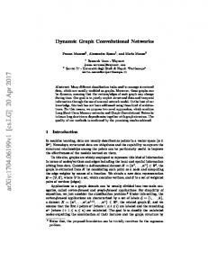
Fig. 1. An overview of our method. The hierarchical context (on three scales) of each pixel is captured spontaneously by a three-column deep convolutional network, which is responsible for predicting the label (person or background) for each pixel of an image.

one often resorts to graph-based methods to capture such relationships. For example, He and Zemel [9] extended the standard conditional random field algorithm to model the relationship between a pixel and its neighbors, namely, to impose spatial smoothness. This can be seen as considering the context of each pixel within a small local region. Limited by the complexity in computation, these sophisticated graph-based methods can hardly capture long range contexts in an image directly. Hierarchical labeling on multiple scales is a way out of this problem [10]. However, the performance still depends on the manually designed hierarchies of segmentations. One natural and elegant way to build the context hierarchy of a pixel is to present a series of patches in raw pixels on different scales (as shown in Fig.1), which allows automatically learning the patterns of contexts to distinguish different kinds of pixels. Unlike classic graph-based methods, convolutional networks can efficiently handle these raw pixel patches, free from the design of segmentation hierarchies. Considering the convincing performance of convolutional networks in terms of image classification and object detection [1], it is natural to anticipate that they can also effectively classify the pixels in an image for the purpose of segmentation. Our proposed method is briefly illustrated in Fig.1. We first densely extract a series of three-level context hierarchies for the pixels in an image, then, each level of the hierarchies is respectively fed into a fivestage convolutional network, which learns the representations of pixels on one level, and finally, a three-layer perceptron is

responsible for predicting the labels of the pixels. In the threelevel hierarchies, contexts within the smallest regions depict the local details, while those within the largest regions captures the object-scene relationships. It should be noted that, Farabet et al. [11] also applied convolutional networks to context patches on three scales in their recent work. However, they did not treat the patches on different scales of the same pixel as a hierarchy from the very beginning. Instead, though their classifier (a two-layer perceptron) is aware of the hierarchical relationships between context patches, their feature extractor (a three-stage convolutional network) is not. In this way, their learned representations are more devoted to tackling with the scale variation of objects, rather than capturing the patterns of hierarchical contexts, which is the very motivation of our scheme. Besides, our proposed method is completely endto-end, which takes raw pixels as the input and outputs the pixel-wise labels without any sophisticated post-processing. Farabet et al. [11] have shown that graph-based post-processing methods can significantly improve the performance of their less deep network with three convolutional stages and a twolayer perceptron. In spite of that, methods with the end-toend feature can benefit from being free of manually designed sophisticated post-processing methods like [11]. The remainder of this paper is organized as follows. The very next section will review more related works about image segmentation and convolutional networks. After that, Section III will describe our method in detail, before the experimental results in Section IV. Finally, this paper will be concluded in Section V. II.

R ELATED W ORK

Conventional approaches to image segmentation are often graph-based such as the conditional random field algorithm. Besides the works by He and Zemel [9] and Ladick´y et al. [10] we have mentioned in the previous section, we name a few more here. Liu et al. [6] proposed a new kind of features named as SIFT Flow and integrated them using the Markov random field (MRF) algorithm. Kumar and Koller [12] applied an accurate linear programming relaxation to their region selection method for speed-up. Lempitsky et al. [13] proposed to flexibly choose the level of segmented regions to label, using their pylon model. Tighe and Lazebnik [8] applied MRF to segmentation over super-pixels. In another recent work, they proposed per-exemplar detectors for image parsing [14], and MRF was used again to smooth predictions. Compared with classic approaches to image segmentation, one of the most attractive characteristics of convolutional neural networks (CNN) would be its ability to be trained in an end-to-end fashion. This brings in great convenience in practical applications. Given sufficient data and labels, CNN can learn an effective model automatically without any handcraft features, either to label new data directly, or to represent them with hierarchical features [15]. More than twenty years ago, LeCun et al. [16] firstly proposed CNN for digit recognition. And now, there are many works based on CNN in the community of computer vision. For example, LeCun et al. [17] applied CNN to object recognition and robot navigating. In the object detection community, Sermanet et al. [18] proposed to learn multi-stage features using unsupervised CNN for pedestrian detection; Ouyang and Wang [19] simulated the

function of the part-based model [20] with CNNs which can jointly learn features, deformation and occlusion. Especially, Krizhevsky et al. [2] has made a breakthrough in large-scale image classification in ILSVRC 2012 [21]. With deep CNNs, they beat the best performer among the classic bag-of-words methods, i.e., Fisher coding [22], with a considerable margin, i.e., about 10% in top-five hit rate. In another task of the same contest, i.e., classification with localization, a revised version of this network also beat the best object detection model, i.e., part-based model [20], with a margin of more than 15%. According to the recently revealed results of ILSVRC 2013 [1], the winners of the three tasks all built up their models based on CNNs. Having won the first place in the newly proposed large-scale object detection task in ILSVRC 2013, CNN has already dominated the first two of the three basic topics, i.e., image classification, object detection and image segmentation. The most related work is the one by Farabet et al. [11]. They used a less deep network, namely, three convolutional stages and two full-connected layers, for the purpose of real-time applications. Experimental results show that deeper networks perform better in our task. Other differences between our method and theirs include the occasion to construct hierarchical contexts and the end-to-end characteristic. More details have been given in the previous section. III.

M ETHOD

We will firstly give an overview of the structure of our networks, then demonstrate the importance of constructing hierarchical contexts early, and finally introduce the details of data preparation and algorithm implementation. A. Overview of the Model The detailed structure of our used network is illustrated in Fig.2. Some of the key parts are listed as follows. 1)

2)

3)

The contexts on three scales of each sampled pixel are respectively fed into the three columns of the network, and the weights are not shared across different columns. Each of the three columns is composed of five convolution stages, wherein the activations of the first and second stages are locally normalized as Krizhevsky et al. [2] did, and the first, second and fifth convolutional layers are followed by spatial pooling layers. A three-layer perceptron is used as the classifier, which takes the representations obtained from the previous three columns as the input. The number of nodes in the last layer is two, since the labels in our used dataset are binary, i.e., person or background [4].

B. Hierarchical Contexts Extracting local patches on multiple scales is one of the common approaches to scale invariance in the community of computer vision. For example, in a typical image classification approach based on the bag-of-words model by Huang et al. [23], local features (SIFT descriptors [24]) are computed on four scales, i.e., 16×16, 24×24, 32×32 and 40×40 in pixels. These local features are then treated equally

Fig. 2. The structure of our network, which is composed of three five-stage convolutional columns and a three-layer perceptron. The details of the second and third columns are omitted, since they are respectively the same as the first column. C: convolution; P: pooling; C1-C5: convolution layers; F1-F3: full-connected layers.

and separately in the next step of the algorithm. In this way, scale invariance is realized on the local feature level. The recent work by Farabet et al. [11] is another example of introducing scale invariance in image labeling using convolutional networks. These schemes worked well for their specific purposes. Besides the scale invariance, we have noticed that a hierarchy which is composed of the patches extracted at the same location can often provide a model with an extra adorable characteristic. The advantage is that the whole model can learn the embedded relationships between contexts on different scales. In this paper, each of the context hierarchies is composed of the three patches centered at the same pixel, as depicted in Fig.2. In the training phase, we attach the label of a pixel to its context hierarchy and feed them into a network. In this way, not only the classifier (a three-layer perceptron) but also the feature extractor (composed of three five-stage convolutional networks) is aware of the embedded relationships in context hierarchies. Otherwise, for example, if we train them in the two-step way proposed by Farabet et al. [11], the feature extractor will lose this characteristic. Farabet et al. trained only one five-stage convolutional network and shared it across different scale columns of the whole network. As a result, the hierarchical contexts are not shown to the feature extractor during training. What we have to do is to use these hierarchies earlier. It is worth noting that our proposed method in this paper does not explicitly ensure scale invariance. However, we can realize that by extracting context hierarchies on multiple scales. In this way, our method can combine the advantages of the two characteristics stated above. We leave this as our future work. C. Data Preparation To eliminate the impact of image sizes, we resize the images in the training set so that their shorter sides are of length 256 in pixels. We then pad the images with a 112-pixel border of zeros, so that it is possible to crop a 224×224 patch centered at any location of an image. In each round of the training phase, we randomly sample a pixel from an image, crop a 224×224 patch which is centered at the sampled pixel. Namely, there are at least 65,536 possible samples in each image. To further enlarge the dataset, we also randomly flip the patches, rescale them with a rate between 0.9 and 1.1 and

rotate them with an angle between -8 and 8 degrees. After that, the RGB values of the patches are centered by subtracting the pixel-wise mean activities on the training set. The last step is to build up the context hierarchies. For a 224×224 patch, we first crop its central 56×56 part to get the smallest context. Secondly, we down-sample the patch into 112×112 with Gaussian blurring, and crop its central 56×56 part to get the second smallest context. Thirdly, we further down-sample the patch into 56×56, so as to get the largest context. Finally, the above three contexts are stacked together to get a hierarchy and fed into our network. D. Implementation Details The details of the three five-stage convolutional networks as illustrated in Fig.2 are similar with the winner of the image classification task in ILSVRC 2012 [21]. The data fed into the network are of the size 56×56. In the first convolutional stage, there are 48 filters of the size 5×5. We pad the input data with a one-pixel border of zeros, so the activations are of the size 54×54, which are normalized across neighboring feature maps following Krizhevsky et al.’s proposal [2]. Overlapping spatial pooling is applied in 3×3 local regions with a stride of two. The second stage is similar with the first one, except that we pad the input data with a two-pixel border and increase the number of filters up to 128. The third and forth stage both have 192 filters of the size 3×3 and are without normalization and pooling layers. The last stage has 64 filters of the size 3×3. Spatial pooling is applied in 3×3 local regions with a stride of two. The classifier (a three-layer perceptron) is also depicted in Fig.2. The two hidden layers both have 1,024 neurons, and the last layer has two, corresponding to the two labels, i.e., person and background, respectively. We use the same activation function (the Rectified Linear Unit) for all the convolution layers and the first two full-connected layers, following Krizhevsky et al.’s proposal [2]. The whole network is trained by back-propagation with the logistic regression loss over the predicted scores normalized using the soft-max function. The weights are initialized using a Gaussian distribution with zero mean and a standard deviation of 0.01. The biases in the forth and fifth convolutional layers, as well as the first two full-connected layers, are initialized with the constant one, while other biases are initialized as zeros. We update all the weights after learning every mini-

batch of the size 128. We start training with a learning rate of 0.01, and reduce it to 0.001 when the performance on the evaluation set stops improving. For all the weights and biases in all layers, the momentum is 0.9, and the weight decay is 0.0005. In the test phase, we use the trained network to predict a 100×100 binary map for each image, and directly resize the map back into the size of the original image as the final segmentation result. Processing ten thousand patches is timeconsuming. It still costs more than one minute per image with parallelization on a GTX Titan GPU. However, fortunately, we can share feature maps across different patches. Since many of them are highly-overlapped with each other, there is no need to recompute all the feature maps for every pixel. With this technique, we can effectively reduce the time cost. IV.

E XPERIMENTAL R ESULTS

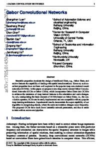
A. Dataset The dataset used in this paper is finely labeled manually for the purpose of foreground segmentation. There are 5,389 images in the training set. Some of them are shown in Fig.3. The task is to segment the most salient person in an image, including his/her clothing, e.g., long dresses and hats, and any objects in his/her hands such as handbags. The images have various sources such as street-shots, advertisements and news. The persons in these images vary greatly in terms of scales and poses. To train our model, we randomly pick out 500 images from the training set for validation. The test set is not public so that no model can be trained using these data. The official evaluation measure is the overlapping rate between ground-truths and predictions averaged over the test set. Mathematically, the score for an image can be formulated as, Ap∩g s= (1) Ap∪g where Ap∩g is the area of the intersection between the groundtruth and the prediction, and Ap∪g is the area of the union of the ground-truth and the prediction. B. Numerical Results To evaluate the impact of hierarchical contexts, we compare three schemes in Tables I. In the first scheme, we crop patches on three different scales from images. In this way, the trained network bears scale invariance. However, neither the feature extractor nor the classifier is aware of the hierarchical relationships between these patches. In the second one, only the classifier is aware of that. In this case, the feature extractor is derived from the trained model of the first scheme and fixed during the subsequent training of the classifier. In the third scheme, both the feature extractor and the classifier can learn the underlying relationships of hierarchical contexts, since we train them spontaneously from raw data. Since the test set is not public, the accuracies listed in Tables I are obtained on our evaluation set. It has 500 images and is excluded from the training set. The improvement gained by hierarchical contexts is smaller than as reported by Farabet et al. [11]. Their two-step training scheme and filter sharing across columns degrade the performance here. This

Fig. 3. Some training samples in Baidu’s dataset for foreground segmentation. Note that the images are reshaped into the same aspect ratio for better viewing.

shows that the results can be affected by various factors, e.g., the specific data and tasks, and the scale of used models. We have to evaluate it case by case. In our specific task, a one-column network with scale invariance performs fine. To further improve the performance, it is a good choice to consider hierarchical contexts early. It is probably vital for the feature extractor to learn the underlying relationships between the contexts on different scales. We list the top four teams in Baidu’s segmentation competition in Table II. The scores are obtained by averaging the overlapping rates of more than one thousand images. According to personal communications, we were the only competitors who used deep learning for segmentation in this contest. One typical method used by the other teams is composed of three steps, i.e., saliency detection, k-NN shape prior and iterative segmentation. Firstly, roughly locate the person in an image using a salient object segmentation method based on context and shape prior [25]. Secondly, find the k-nearest neighbors of an image in the training set, measured by the masks obtained in the first step, and average the masks of the k neighbors so as to update the one of the image. Thirdly, clean up the boundaries and make the decision using graph-based methods such as graph-cut. Run the second and third steps alternatively until the algorithm converges. The results show that our method outperforms the second place team by more than 8%. Note the drastic variations in scales and poses shown in Fig.3. Probably, our deep network with a large number of parameters (about ten million) has the potential to learn the complicated patterns for image segmentation. C. Qualitative Results The segmentation results obtained on Baidu’s test set are given in Fig.4. The results show that our method is robust to complex backgrounds (the eight samples in the left-most column) and variations in poses (the second column) and

Fig. 4.

Segmentation results obtained on Baidu’s test set under various conditions. To the right of each image are in turn its ground-truth and our result. Method No hierarchies Late hierarchies Early hierarchies

Accuracy (%) 85.0 85.3 86.7

TABLE I.

C OMPARISON WITH DIFFERENT METHODS , EVALUATED ON OUR VALIDATION SET. S EE THE TEXT FOR MORE DETAILS . Team Second place Third place Forth place Ours

TABLE II.

Accuracy (%) 78.17 76.00 75.95 86.83

C OMPARISON WITH OTHER

COMPETITORS

[4].

scales (the third). The eight samples in the right-most column show that our method can also effectively find various objects in hands. As shown in Fig.5, most of the failed cases are due to confusing backgrounds. However, there is room for improvement. Note that we directly reshape the 100×100 predicting map of an image back to the original size, without any post-processing. As a result, there might be multiple separated regions in our predictions. Trivial post-processing approaches such as removing small foreground regions can alleviate the impact of this problem. More sophisticated postprocessing can be adopted either to smooth the boundaries or ensure consistent labeling [11]. We leave these as our future work.

Fig. 5.

Hard samples in Baidu’s test set.

V.

C ONCLUSION

In this paper, we have proposed an image segmentation method based on deep convolutional networks, which is com-

posed of a three-column feature extractor and a classifier. By early stacking together the contexts on multiple scales of the pixels in an image, we have trained feature extractors which are aware of the hierarchical relationships between contexts on different scales. Experiments have shown that early-combining is better than late-combining given the conditions in this paper. Our method has outperformed classic segmentation methods with a considerable margin. Furthermore, qualitative results have shown that our method is close to practical application. ACKNOWLEDGMENT Thanks to Weiqiang Ren for his hard work to contribute a CPU implementation of CUDA-convnet. This work is jointly supported by National Basic Research Program of China (2012CB316300) and National Natural Science Foundation of China (61135002, 61175003, 61203252). R EFERENCES [1] O. Russakovsky, J. Deng, J. Krause, A. Berg, and F. Li, “ImageNet Large Scale Visual Rcognition Challenge 2013 (ILSVRC 2013),” 2013. [2] A. Krizhevsky, I. Sutskever, and G. Hinton, “ImageNet classification with deep convolutional neural networks,” in NIPS, 2012. [3] M. Everingham, L. Van Gool, C. K. I. Williams, J. Winn, and A. Zisserman, “The PASCAL Visual Object Classes Challenge 2007 (VOC2007) Results,” 2007. [4] Baidu, “Baidu Context Dataset 2013,” http://openresearch.baidu.com/ activityprogress.jhtml?channelId=576, 2013. [5] Z. He, T. Tan, Z. Sun, and X. Qiu, “Towards accurate and fast iris segmentation for iris biometrics,” IEEE Trans. Pattern Analysis and Machine Intelligence, vol. 31, pp. 1670–1684, 2008. [6] C. Liu, J. Yuen, and A. Torralba, “Nonparametric scene parsing: Label transfer via dense scene alignment,” in CVPR, 2009. [7] B. Russell, A. Torralba, C. Liu, R. Fergus, and W. Freeman, “Object recognition by scene alignment,” in NIPS, 2007. [8] J. Tighe and S. Lazebnik, “SuperParsing: Scalable nonparametric image parsing with superpixels,” in ECCV, 2010. [9] X. He and R. Zemel, “Learning hybrid models for image annotation with partially labeled data,” in NIPS, 2008. [10] L. Ladick´y, C. Russell, and P. Kohli, “Associative hierarchical CRFs for object class image segmentation,” in ICCV, 2009. [11] C. Farabet, C. Couprie, L. Najman, and Y. LeCun, “Learning hierarchical features for scene labeling,” IEEE Trans. Pattern Analysis and Machine Intelligence, 2013. [12] M. Kumar and D. Koller, “Efficiently selecting regions for scene understanding,” in CVPR, 2010. [13] V. Lempitsky, A. Vedaldi, and A. Zisserman, “A pylon model for semantic segmentation,” in NIPS, 2011. [14] J. Tighe and S. Lazebnik, “Finding things: Image parsing with regions and per-exemplar detectors,” in CVPR, 2013. [15] P. Sermanet, S. Chintala, and Y. LeCun, “Convolutional neural networks applied to house numbers digit classification,” in ICPR, 2012. [16] Y. LeCun, B. Boser, J. Denker, and D. Henderson, “Handwritten digit recognition with a back-propagation network,” in NIPS, 1989. [17] Y. LeCun, K. Kavukvuoglu, and C. Farabet, “Convolutional networks and applications in vision,” in International Symposium on Circuits and Systems, 2010. [18] P. Sermanet, K. Kavukcuoglu, S. Chintala, and Y. LeCun, “Pedestrian detection with unsupervised multi-stage feature learning,” in CVPR, 2013. [19] W. Ouyang and X. Wang, “Joint deep learning for pedestrian detection,” in CVPR, 2013. [20] P. Felzenszwalb, R. Girshick, D. McAllester, and D. Ramanan, “Object detection with discriminatively trained part-based models,” IEEE Trans. Pattern Analysis and Machine Intelligence, vol. 32, pp. 1627–1645, 2010.

[21] J. Deng, A. Berg, S. Satheesh, H. Su, A. Khosla, and F. Li, “ImageNet Large Scale Visual Rcognition Challenge 2012 (ILSVRC 2012),” 2012. [22] F. Perronnin, J. S´anchez, and T. Mensink, “Improving the Fisher kernel for large-scale image classification,” in ECCV, 2010. [23] Y. Huang, Z. Wu, L. Wang, and T. Tan, “Feature coding in image classification: A comprehensive study,” IEEE Trans. Pattern Analysis and Machine Intelligence, 2013. [24] D. G. Lowe, “Distinctive image features from scale-invariant keypoints,” International Journal of Computer Vision, vol. 2(60), pp. 91–110, Jan. 2004. [25] H. Jiang, J. Wang, Z. Yuan, T. Liu, N. Zheng, and S. Li, “Automatic salient object segmentation based on context and shape prior,” in BMVC, 2011.