stanford.edu). C. F. Beaulieu, D. S. Paik, R. B. Jeffrey, Jr., ..... [4] C. D. Johnson and A. H. Dachman, âCT colonography: The next colon screening examination?
IEEE TRANSACTIONS ON MEDICAL IMAGING, VOL. 21, NO. 12, DECEMBER 2002
1461
Edge Displacement Field-Based Classification for Improved Detection of Polyps in CT Colonography Burak Acar*, Christopher F. Beaulieu, Salih B. Göktürk, Carlo Tomasi, David S. Paik, R. Brooke Jeffrey, Jr., Judy Yee, and Sandy Napel
Abstract—Colorectal cancer can easily be prevented provided that the precursors to tumors, small colonic polyps, are detected and removed. Currently, the only definitive examination of the colon is fiber-optic colonoscopy, which is invasive and expensive. Computed tomographic colonography (CTC) is potentially a less costly and less invasive alternative to FOC. It would be desirable to have computer-aided detection (CAD) algorithms to examine the large amount of data CTC provides. Most current CAD algorithms have high false positive rates at the required sensitivity levels. We developed and evaluated a postprocessing algorithm to decrease the false positive rate of such a CAD method without sacrificing sensitivity. Our method attempts to model the way a radiologist recognizes a polyp while scrolling a cross-sectional plane through three-dimensional computed tomography data by classification of the changes in the location of the edges in the two-dimensional plane. We performed a tenfold cross-validation study to assess its performance using sensitivity/specificity analysis on data from 48 patients. The mean specificity over all experiments increased from 0.19 (0.35) to 0.47 (0.56) for a sensitivity of 1.00 (0.95). Index Terms—Computed tomographic colonography (CTC), computer-aided diagnosis, edge displacement fields (EDFs), fiber-optic colonoscopy (FOC).
I. INTRODUCTION
C
OMPUTED tomographic colonography (CTC) was first suggested in the early 1980s as a potential method for mass screening of colorectal cancer, the second leading cause of cancer deaths in the US [1], [2]. CTC was first realized in the 1990s following the rapid progress in computed tomography (CT) and in digital computing [3]–[5]. CTC is a minimally invasive method that consists of CT imaging the whole abdomen and pelvis after cleansing and air insufflation of the colon. Since then, several studies have been conducted assessing the
Manuscript received July 1, 2001; revised July 29, 2002. This work was supported in part by the National Institutes of Health under Grant 1R01 CA72023 and in part by grants from The Lucas Foundation, The Packard Foundation, and The Phil N. Allen Trust. The Associate Editor responsible for coordinating the review of this paper and recommending its publication was M. Giger. Asterisk indicates corresponding author. *B. Acar is with the Department of Radiology, LUCAS MRS Center, 3D Laboratory, Stanford University, Stanford, CA 94305 USA (e-mail: bacar@ stanford.edu). C. F. Beaulieu, D. S. Paik, R. B. Jeffrey, Jr., and S. Napel are with the Department of Radiology, LUCAS MRS Center, Stanford University, Stanford, CA 94305 USA. S. B. Göktürk and C. Tomasi are with the Department of Electrical Engineering and Computer Science, Stanford University, Stanford, CA 94305 USA. J. Yee is with the San Francisco Veterans Administration Medical Center, University of California, San Francisco, CA 94121 USA. Digital Object Identifier 10.1109/TMI.2002.806405
performance of CTC [6]–[11], mostly based on a radiologist’s visual examination of either two-dimensional (2-D) CT images or three-dimensional (3-D) virtual colonoscopic views, or both. Thus, most efforts have been directed toward developing better visualization and navigation techniques, such as rendering, colon wall flattening, flight path planning algorithms, and user interface design [5], [12]–[20]. However, recently some research has been focused on developing computer-aided detection (CAD) methods for the identification of colonic polyps in 3-D CT data to improve the accuracy and efficiency of CTC. In most approaches, the 3-D geometrical features of polyps are extracted and used for their detection and identification. Mir et al. reviewed a set of methods proposed for shape description in CT images, e.g., moments, medial axis transforms, splines, curvature, Fourier descriptors, AR modeling, and statistical approaches [21]. Summers et al. concluded that detection by shape analysis is feasible, especially for clinically important large polyps [22], [23]. Paik et al. proposed to use a Hough transform (HT)-based method to detect spherical surface patches along the colon wall that are likely to be parts of polyps [24], [25]. Yoshida et al. reported that geometric features extracted from small volumes of interest are effective in differentiating polyps from folds and feces [26], as well as characterizing colon wall surface geometry [35]. Göktürk et al. fitted local spheres to the colon wall and based their detection on the existence of clusters of sphere centers [27]. The main weakness of most of these methods is their low specificity. As a result, manual examination of a large number of images corresponding to the CAD outputs is required. Our goal is to develop and evaluate a postprocessing algorithm that would classify the outputs of a high-sensitivity low-specificity CAD method to eliminate false positives only, thus to increase specificity without sacrificing sensitivity. We used the HT-based CAD (HTD) as the initial detection method [24], [25], and developed a second stage that models the way a radiologist recognizes a polyp by focusing on the changes in consecutive images as one views sequential cross sections of the volumetric source CT data (3-D CT data). We used edge displacement fields (EDFs) to represent these features, and a linear classifier acting on the features extracted from the computed EDFs. A different approach with the same goals has recently been proposed by our group, which uses a large number of cross-sectional images of suspicious structures and the histogram of 2-D image features extracted from them [28]. We evaluated our method using data from 48 patients, and assessed the improvement in the specificity at given sensitivity levels.
0278-0062/02$17.00 © 2002 IEEE
1462
IEEE TRANSACTIONS ON MEDICAL IMAGING, VOL. 21, NO. 12, DECEMBER 2002
Fig. 1. Generation of an axial EDF demonstrated using a hypothetical sphere. The predetected suspicious structure (the sphere) is sliced perpendicular to the scrolling axis (in this case, the z axis). The differential changes in the grayscale image on each slice are computed using (1), with the positive z direction defined to be outwards from the center slice. EDFs v (x; y ) computed for each slice are added and smoothed to get a single EDF v (x; y ) (Z = Axial in this example) representative of the interslice image relations along the z axis. The PN is marked with a square and the CNs are marked with circles. The whole process is repeated for the x and y axes to generate the sagittal and coronal EDFs, respectively.
II. METHODS A. Algorithm We used our previously developed software to identify structures that are suspected of being polyps. Briefly, the software first segments the colon from the rectum to the cecum using gray-level thresholding [19]. It next identifies the colon wall by dilation and determination of intensity gradients, and uses an HT-based polyp detector (the HTD) to detect spherical surface patches (polyp-like structures) within a thin shell surrounding the colon wall [24], [25]. The HTD produces a score for each voxel that is proportional to the number of vectors normal to the colon wall and extending 5 mm into the tissue that intersect the voxel. Intuitively, the voxels close to the center of a spherical surface patch would have a high HT score. We defined the voxels with an HT score larger than 3000 (an arbitrary but low threshold) to be the HTD detected points (HT_hits). HT_hits closer than 10 mm to each other were considered to be marking the same spherical surface patch, so they were replaced with a single HT_hit, that is, their maximum. We extracted subvolumes of 21 21 21 voxels (mean size 15.6 mm 15.6 mm 26.9 mm) centered at the HT_hits and postprocessed them with our EDF-based classifier (EDFC). The first step of postprocessing is the EDF computation to represent the changes in the location of edges in the segmented CT images (tissue/air boundaries) as one scrolls through the 3-D CT data. We consider three mutually orthogonal scrolling axes perpendicular to axial, coronal, and sagittal planes, as follows. Let the plane be an image plane perpendicular to the scrolling Axial, Sagittal, Coronal . The EDF equation is [29] axis (1) is the EDF (2-D in-plane vector field) where defined on the plane that is perpendicular to the axis and . is the associated image, is located at that i.e., the attenuation coefficient function on the same plane. represents the dislocation of the edge at along the local gradient from to . is computed for all , i.e., for all slices, within the subvolume except at the boundaries. We defined the positive direction
to be outwards from the center slice. This consistency is required as for all are summed and smoothed to , associated with the current get a composite EDF, (see Fig. 1). Thus, it is subvolume and the scrolling axis assured that the edges of polyp-like structures move inwards on the plane perpendicular to the scrolling axis. The composite EDF is smoothed. The smoothing kernel is a Gaussian mm) whose size is limited to . This is repeated ( Axial, Sagittal, Coronal ) for all three orthogonal axes ( resulting in three EDFs that encode information in each of , them. In the following, the term EDF will refer to , or . The second step is to characterize the computed EDFs. To characterize a single EDF, one parent node (PN) and eight child nodes (CNs) are determined. A PN is defined to be the minimum divergence pixel location in a 4 mm 4 mm neighborhood of the HT_hit on the EDF. CNs are defined to be the pixel locations that are 4 mm away from the PN on the streamlines incoming to the eight immediate neighbors of the PN. The right side of Fig. 1 depicts the process graphically. Fig. 2 shows an actual example with three associated axial images. Two parameters, and , are computed using the Jacobian matrix of the EDF at the PN, as follows [30], [31]:
(2) (3) (4) Note that and carry information about the eigenvalues of the Jacobian matrix . In fact, the characteristic equation of is (5) Furthermore, is equal to the divergence of the EDF at PN. The ratio of to uniquely defines the topology of a linear vector ) are field so the normalized and (normalized by used as suggested by Lavin et al. [31].
ACAR et al.: EDGE DISPLACEMENT FIELD-BASED CLASSIFICATION FOR IMPROVED DETECTION OF POLYPS IN CTC
Fig. 2. Three sequential axial images (smoothed for visual purposes) around (x; y ). The PN is marked with a an HT_hit and the associated EDF v square and the CNs are marked with small circles. Two of the eight CNs are coincident with two other CNs.
Additionally, we characterize the behavior of the incoming streamlines around the PN using the parameter , defined as
1463
(a)
(b)
(c)
(d)
�; ; d
Fig. 3. Axial EDFs of four cases: (a) positive (polyp) with [ ] = ] = [ 0 99 0 12 5 15]; [ 0 96 0 29 4 99]; (b) positive with [ (c) negative (nonpolyp) [ ] = [ 0 77 0 65 1 28]; (d) negative with [ ] = [ 0 71 0 70 072].
0: ; : ; : �; ; d �; ; d 0: ; : ;
�; ; d 0: ; : ; :
0: ; : ; :
Mahalanobis distance of a vector to the mean vector population is defined as
of a
(7) (6) where the s are computed with respect to the PN’s location. Thus, is used to characterize the spread of CNs around the PN. Fig. 3 shows four axial EDFs computed for two positive (polyp) and two negative (nonpolyp) cases to give an understanding of the meaning of EDF characterization parameters visually. In agreement with the intuition, the EDFs corresponding to positive cases have a PN with an close to 1 (negative divergence) and close to zero (small circulatory behavior), and a large (streamlines well spread around the PN), i.e., a star-shaped topology, unlike the EDFs of negative cases. Each parameter is computed for the axial, coronal, and sagittal EDFs, resulting in a nine-dimensional feature vector for each subvolume considered. We selected to use the mean values of each parameter over three scrolling axes as the final feature vector. This choice is based on a previous study where we have shown, on a smaller data set, that this choice results in marginally better classification than a range of other choices [32]. In the rest, we will refer to this definition, i.e., , where stands for averaging over axial, coronal, and sagittal parameters. The binary classification (polyp versus nonpolyp) is done by a Mahalanobis distance based linear classifier [33]. The
is the covariance matrix of . This distance is a stanwhere dardized measure that: 1) automatically accounts for scaling; 2) takes care of correlations between features; and 3) can provide linear and curved decision surfaces. For classification purposes, represents the training set and represents a sample from the test set . Referring to the subset of polyps in as and the subset of nonpolyps as , the binary classifier is defined as follows:
otherwise
(8)
and refer to the subsets of polyps and nonpolyps where in . All processing was done using Matlab 6.0 (The Mathworks Inc., Natick, MA). In addition, the time required to process individual subvolumes was measured using Matlab’s tic/toc commands. B. Evaluation The CTC data were acquired from 48 patients enrolled in 12), our CTC study (45 male, age 27–86, mean age 60 either in the supine or the prone position, following colon cleansing and air insufflation. A single- or multidetector CT system (GE Medical Systems, Milwaukee, WI) was used with
1464
IEEE TRANSACTIONS ON MEDICAL IMAGING, VOL. 21, NO. 12, DECEMBER 2002
Fig. 4. SS and SS curves for each of ten experiments. Solid line (—) is the two-stage system, HTD followed by EDFC; dashed line (- -) is the single-stage system, HTD only.
the following parameters: 3 mm (2.5 mm) collimation, pitch 1.5–2.0 (3.0), 1.5 mm (1.0–1.5 mm) reconstruction interval, 120 kVp (120 kVp), 200 mAs (56 mAs) for the single- (multi) where detector system. The data size was ranged from 237 to 403. The the number of axial slices average voxel spacing was 0.74 mm 0.74 mm 1.28 mm. All of the patients underwent fiber-optic colonoscopy (FOC) immediately after the CTC. Preprocessing with HTD resulted in 31 099 HT_hits. An expert radiologist, unblinded to the FOC results, examined the CTC images and reconciled the FOC determined lesions with CTC visibility. Due to computational concerns, we subsampled the data set by keeping all polyps (i.e., positives) and randomly selecting 50 nonpolyps (i.e., negatives) per patient, uniformly distributed over the range of HT scores for each patient. The radiologist then eliminated any multiple HT_hits for a single polyp by including the one closest to the coordinates determined manually on CTC data. A colonic cancer of 32 mm in diameter was excluded in accordance with our aim of detecting polyps. The HT_hits that were annotated as polyps by both FOC and CTC were designated as positives. Similarly, the HT_hits that were not annotated as polyps by FOC or by CTC were designated negatives. These served as the gold standard. There were 46 positives and 2400 negatives in the preprocessed data set. Six positives and 181 negatives were excluded due to their closeness to the volume boundary, in which case the subvolume required for processing could not be extracted. This resulted in a final data set of 40 positives (sizes ranging from 2 to 15 mm) and 2219 negatives. The subvolumes centered at each of the 2259 HT_hits were used as the input data to the EDFC. To evaluate our system, we performed a tenfold cross-validation study. We distributed 40 positives into ten sets, each containing ten distinct positives by using 20 randomly selected positives twice and the rest three times. The average overlap in positives between all pairs of sets is 1.8; the maximum overlap is 4 (which is in two pairs only). In these ten sets, 2219 negatives were randomly distributed mutually exclusively by putting 221 negatives in one set and 222 negatives in the others. Thus, each set contained ten distinct positives (polyps) and 221 or
222 distinct negatives (nonpolyps). For each experiment, one such set was used as the test set and the union of the remaining sets was used as the training set. Thus, we had 30 positives and 1997 (or 1998) negatives in each training set. The sensitivity and the specificity were defined as the percentage of correctly identified positives and negatives, respectively, in the test set. The principal question we addressed was How much can we increase the specificity of a detector by postprocessing its outputs, without sacrificing sensitivity? To answer this question, we performed the following analysis. For each of the ten experiments, we ran the HTD and classified its output by varying on HT Score . Varying in this way genthe range curve relating (sensitivity of HTD alone) erates the (specificity of HTD alone). Next, for each , we apto plied the EDFC to the positives identified by the HTD, varying [see (8)] across its entire range for this experiment. Varying in this way generates a curve relating (sensitivity of HTD (specificity of HTD and and EDFC combined) to EDFC combined) at this particular . Note that because only the set of positive outputs of the HTD (which is a function of ) are passed to the EDFC, the EDFC cannot lower the specificity. On each of these curves, we determined the maximum specificity at the sensitivity level set by HTD alone at the corresponding . (Equivalently, this point is the maximum specificity at 100% sensitivity on the curve that is parameterized by , at that .) to mean the sensitivity of HTD alone and the Thus, we use sensitivity of the combination HTD and EDFC. Concatenation of these points provides us another sensitivity/specificity curve ). ( and curves for ten We report each of the is, by definition, always experiments (see Fig. 4). because a postprocessing method cannot deto the left of crease the specificity, i.e., cannot create new false positives that are not included in the set of data predicted to be positive by and provides a simple HTD. Comparison of way to answer the question we put forth above. The differences in specificity levels at a given sensitivity level (the horizontal and ) shows the improveseparation between ment in specificity achieved by EDFC at that sensitivity. We de-
ACAR et al.: EDGE DISPLACEMENT FIELD-BASED CLASSIFICATION FOR IMPROVED DETECTION OF POLYPS IN CTC
TABLE I MEAN
AND STANDARD DEVIATION OF MAXIMUM SPECIFICITY LEVELS ACHIEVED BY ONE-STAGE (HT) AND TWO-STAGE (HT EDF) METHODS AT DIFFERENT SENSITIVITY LEVELS SET BY THE FIRST STAGE. CORRESPONDING TWO-TAILED VALUES ARE COMPUTED BY PAIRED TESTS WITH THE NULL HYPOTHESIS THAT THE DIFFERENCE OF THE MEANS OF AND OVER TEN EXPERIMENTS IS ZERO
+
p
t
Sp
Sp
termined the maximum s and s for a number of sensitivity levels each of which corresponds to different operating points set by . Due to the discrete nature of the and curves, we approximated the 95% sensitivity point by linearly interpolating the maximum specificity points for 100% and 90% sensitivity levels. The statistical significance of the difference between the mean specificity levels at different sensitivity levels was also assessed. We computed the two-tailed values of the paired tests performed on the sets of maximum and values at different sensitivity levels. The null hypothesis was and is zero that the difference of the means of over ten experiments. The mean and the standard deviation of specificity values and the corresponding values are reported. III. RESULTS Table I lists the mean and the standard deviation of the maximum specificity values for one- and two-stage methods at different sensitivity levels set by the HTD’s threshold . The corresponding values assess the significance of the difference between these mean values, based on ten cross-validation experiments. The mean improvements in specificity at clinically relevant sensitivity values, i.e., at 1.00 and 0.95 sensitivity levels, 0.12 to 0.47 0.16) and 0.21 (from are 0.28 (from 0.19 0.35 0.13 to 0.56 0.14) with values of 4.7 10 and 2.2 10 , respectively. The improvement in specificity is sig) for sensitivity levels larger than 0.50. nificant ( The computation time for a single subvolume on a PC with Pentium III processor (1-GHz clock rate), 512-MB RAM, using Matlab 6.0, was 3.0 s on the average. There were approximately
1465
600 HT_hits per patient; thus, the analysis of a single patient would require 30 min. IV. DISCUSSION The low specificity of previously reported CAD methods is generally due to the assumption that high curvature surface patches occur only on polyps. While it is true that polyps have highly curved surfaces, so do some other structures, like haustral folds and retained stool. Radiologists reading these scans use additional information with which they classify suspicious regions. For example, haustral folds are elongated structures, as opposed to polyps, which protrude locally from the colon wall. Stool may sometimes be identified by relatively inhomogeneous image intensity compared to polyps. The approach pursued in this study was to model the way a radiologist discriminates these structures while scrolling a cross-sectional plane (the image plane) through the 3-D CT data. Our algorithm is based on quantitative evaluation of the changes in local image gradients in consecutive image planes. These gradients mainly capture the information in air/tissue boundaries (the edges). As one moves through a series of image planes, the edges of elongated structures (such as haustral folds) are likely to sweep a large portion of the image plane, whereas those of locally protruding structures (such as polyps) are likely to appear/disappear instantaneously at some image plane. The EDFs, computed as described above, are aimed to capture this property. As a conjecture, we expect the summation and smoothing operations help to enhance the difference between homogeneous and inhomogeneous structures (such as polyps and stool). In case of inhomogeneous structures, the contribution of the local image gradients at pixels other than the edges would be more significant than it would be for a homogeneous structure. Furthermore, this contribution would be in a relatively random fashion, canceling the contribution from the edges and, thus, enhancing the discrimination between spherical homogeneous and inhomogeneous structures. This conjecture remains to be studied. The inherent assumption in our method is that the majority of the EDFs around polyps along different scrolling axes will be similar to the EDFs of positive cases in Fig. 3, whereas this will not be the case around nonpolyps. Our choice of averaging the parameters over three image planes is based on this assumption and our previous study that showed no significant sensitivity of the performance to different choices, such as minimum, maximum, median, etc. [32]. However, this averaging may still introduce too much smoothing to the parameters, degrading the performance. A better approach might be to make measurements in a large number of scrolling axes and to use the resulting parameters in the form of a histogram. However, in this study we aimed to model a radiologist’s classification task and, therefore, confined our analysis to the data most easily available to a radiologist, namely, to three orthogonal image planes. Another alternative is to use the EDFs in the vicinity of PNs as they are, without extracting single parameters (e.g., , , ) from them. Support vector machines (SVMs) can be trained to learn from these EDFs [34]. The critical point is to design an appropriate
1466
IEEE TRANSACTIONS ON MEDICAL IMAGING, VOL. 21, NO. 12, DECEMBER 2002
SVM kernel that will capture the relevant information in these EDFs. The sensitivity of our algorithm to polyps of different sizes depends on the voxel size and the size of the subvolume considered. The parameters we used in this study support the representation of structures up to 15.5 mm 15.5 mm 26.9 mm large on the average. An increase in the EDFs’ discriminative power with a decrease in voxel size is expected. We excluded the HT_hits close to the volume boundary for the sake of analysis in this study. Such an exclusion can be avoided by defining the CNs to be on the volume boundary if the streamlines, on which the CNs are located, hit the volume boundary before the preset distance, which is 4 mm. The PNs, on the other hand, cannot be on the volume boundary as they are on the colon wall by definition. The computational analysis for a single patient with approximately 600 HT_hits required approximately 30 min. While Matlab is an excellent prototyping environment, we would expect significant time reductions with optimized software. Thus, we do not expect our method to be a rate-limiting step in clinical practice. V. CONCLUSION We have shown that the information content of the motion of edges (air/tissue boundary) in sequential cross sections through the 3-D CTC data is relevant in polyp identification and that the use of EDFs is adequate to represent this information. The intuitive nature of the proposed EDF characterization parameters ( , , ) make it easy to interpret the feature vectors: As and decrease and increases, the “polypness” of the structure increases. Although a statistically significant improvement in specificity is achievable at clinically relevant sensitivity levels, these specificity levels are still too low for clinical applications. The method is limited by the number of image planes (currently, three) and the performance of the classifier. The method assumes that the predetected points are sufficiently close to the geometrical center of the suspicious structures, which may be limiting the performance of EDFC. Increasing the number of image planes and constructing a histogram of the parameters would remove this assumption and is subject to future research. An alternative to the Mahalanobis distance-based classifier is the use of SVMs, which minimize training classification error as well as generalization error. Higher specificity levels are required for practical clinical applications and we believe that the above-mentioned improvements would achieve this. ACKNOWLEDGMENT The authors would like to thank R. Prokesch for his contributions at the clinical phase of this study. REFERENCES [1] C. G. Coin, F. C. Wollett, J. T. Coin, M. Rowland, R. K. Deramos, and R. Dandrea, “Computerized radiology of the colon: A potential screening technique,” Comput. Radiol., vol. 7, no. 4, pp. 215–221, 1983. [2] P. J. Wingo, “Cancer statistics,” CA—Cancer J. Clinicians, vol. 45, pp. 8–30, 1995.
[3] A. S. Chaoui, M. A. Blake, M. A. Barish, and H. M. Fenlon, “Virtual colonoscopy and colorectal cancer screening,” Abdom. Imag., vol. 25, no. 2, pp. 361–367, 2000. [4] C. D. Johnson and A. H. Dachman, “CT colonography: The next colon screening examination?,” Radiology, vol. 216, no. 2, pp. 331–341, 2000. [5] D. J. Vining, “Virtual colonoscopy,” Gastrointest. Endosc. Clin. North Amer., vol. 7, no. 2, pp. 285–291, 1997. [6] A. K. Hara, C. D. Johnson, J. E. Reed, D. A. Ahlquist, H. Nelson, R. L. Ehman, C. H. McCollough, and D. M. Ilstrup, “Detection of colorectal polyps by computed tomographic colography: Feasibility of a novel technique,” Gastroenterol., vol. 110, no. 1, pp. 284–290, 1996. [7] M. Macari, A. Milano, M. Lavelle, P. Berman, and A. J. Megibow, “Comparison of time-efficient CT colonography with two- and three-dimensional colonic evaluation for detecting colorectal polyps,” Amer. J. Roentgenol., vol. 174, no. 6, pp. 1543–1549, 2000. [8] A. K. Hara, C. D. Johnson, J. E. Reed, D. A. Ahlquist, H. Nelson, R. L. MacCarty, W. S. Harmsen, and D. M. Ilstrup, “Detection of colorectal polyps with CT colography: Initial assessment of sensitivity and specificity,” Radiology, vol. 205, no. 1, pp. 59–65, 1997. [9] D. K. Rex, D. Vining, and K. K. Kopecky, “An initial experience with screening for colon polyps using spiral CT with and without CT colography,” Gastrointest. Endosc., vol. 50, no. 3, pp. 309–313, 1999. [10] American Society for Gastrointestinal Endoscopy ASGE, “Technology status evaluation: Virtual colonoscopy: November 1997,” Gastrointest. Endosc., vol. 48, no. 6, pp. 708–710, 1998. [11] A. H. Dachman, J. K. Kuniyoshi, C. M. Boyle, Y. Samara, K. R. Hoffmann, D. T. Rubin, and I. Hanan, “CT colonography with three-dimensional problem solving for detection of colonic polyps,” Amer. J. Roentgenol., vol. 171, no. 4, pp. 989–995, 1998. [12] D. S. Paik, C. F. Beaulieu, R. B. Jeffrey, C. A. Karadi, and S. Napel, “Visualization modes for CT colonography using cylindrical and planar map projections,” J. Comput. Assist. Tomogr., vol. 24, no. 2, pp. 179–188, 2000. [13] C. L. Kay, D. Kulling, R. H. Hawes, J. W. R. Young, and P. B. Cotton, “Virtual endoscopy—Comparison with colonoscopy in the detection of space-occupying lesions of the colon,” Endoscopy, vol. 32, no. 3, pp. 226–232, 2000. [14] T. Y. Lee, P. H. Lin, C. H. Lin, Y. N. Sun, and X. Z. Lin, “Interactive 3-D virtual colonoscopy system,” IEEE Trans. Inform. Tech. Biomed., vol. 3, pp. 139–150, June 1999. [15] C. F. Beaulieu, Jr., R. B. Jeffrey, C. Karadi, D. S. Paik, and S. Napel, “Display modes for CT colonography, Part II. Blinded comparison of axial CT and virtual endoscopic and panoramic endoscopic volume-rendered studies,” Radiology, vol. 212, no. 1, pp. 203–212, 1999. [16] G. Wang, E. G. McFarland, B. P. Brown, and M. W. Vannier, “GI tract unraveling with curved cross sections,” IEEE Trans. Med. Imag., vol. 17, pp. 318–322, Feb. 1998. [17] E. G. McFarland, J. A. Brink, J. Loh, G. Wang, V. Argiro, D. M. Balfe, J. P. Heiken, and M. W. Vannier, “Visualization of colorectal polyps with spiral CT colography: Evaluation of processing parameters with perpective volume rendering,” Radiology, vol. 205, no. 3, pp. 701–707, 1997. [18] S. Haker, S. Angenent, A. Tannenbaum, and R. Kikinis, “Nondistorting flattening maps and the 3-D visualization of colon CT images,” IEEE Trans. Med. Imag., vol. 19, pp. 665–670, Dec. 2000. [19] D. S. Paik, C. F. Beaulieu, R. B. Jeffrey, G. D. Rubin, and S. Napel, “Automated flight path planning for virtual endoscopy,” Med. Phys., vol. 25, no. 5, pp. 629–637, 1998. [20] Y. Samara, M. Fiebich, A. H. Dachman, J. K. Kuniyoshi, K. Doi, and K. R. Hoffmann, “Automated calculation of the centerline of the human colon on CT images,” Acad. Radiol., vol. 6, no. 6, pp. 352–359, 1999. [21] A. H. Mir, M. Hanmandlu, and S. N. Tandon, “Description of shapes in CT images: The usefulness of time-series modeling techniques for identifying organs,” IEEE Eng. Med. Biol. Mag., vol. 18, pp. 79–84, Jan./Feb. 1999. [22] R. M. Summers, C. F. Beaulieu, L. M. Pusanik, J. D. Malley, R. B. Jeffrey, D. I. Glazer, and S. Napel, “Automated polyp detector for CT colonography: Feasibility study,” Radiology, vol. 216, no. 1, pp. 284–290, 2000. [23] R. M. Summers, C. D. Johnson, L. M. Pusanik, J. D. Malley, A. M. Youssef, and J. E. Reed, “Automated polyp detection at CT colonography: Feasibility assessment in a human population,” Radiology, vol. 219, no. 1, pp. 51–59, 2001. [24] D. S. Paik, C. F. Beaulieu, R. B. Jeffrey, J. Yee, A. M. Steinauer-Gebauer, and S. Napel, “Computer-aided detection of polyps in CT colonography: Free response ROC evaluation of performance,” Radiology, vol. 217(SS), p. 370, 2000.
ACAR et al.: EDGE DISPLACEMENT FIELD-BASED CLASSIFICATION FOR IMPROVED DETECTION OF POLYPS IN CTC
[25] D. S. Paik, C. F. Beaulieu, R. B. Jeffrey, C. Karadi, and S. Napel, “Detection of polyps in CT colonography: A comparison of a computer aided detection algorithm to 3-D visualization methods,” in Proc. 85th Scientific Sessions Radiological Society of North America, vol. 213(P). Chicago, IL, 1999, p. 428. [26] H. Yoshida, Y. Masutani, P. M. MacEneaney, K. Doi, Y. Kim, and A. H. Dachman, “Detection of colonic polyps in CT colonography based on geometric features,” Radiology, vol. 217(SS), p. 582, 2000. [27] S. B. Göktürk and C. Tomasi, “A graph method for the conservative detection of polyps in the colon,” in Proc. 2nd Int. Symp. Virtual Colonoscopy, Boston, MA, 2000. [28] S. B. Göktürk, C. Tomasi, B. Acar, C. F. Beaulieu, D. Paik, Jr., R. B. Jeffrey, J. Yee, and S. Napel, “A statistical 3-D pattern processing method for computer aided detection of polyps in CT colonography,” IEEE Trans. Med. Imag., vol. 20, pp. 1251–1260, Dec. 2001. [29] S. S. Beauchemin and J. L. Barron, “The computation of optical flow,” Comput. Surv., vol. 27, no. 3, pp. 433–467, 1995. [30] J. Helman and L. Hesselink, “Representation and display of vector field topology in fluid flow data sets,” IEEE Computer, vol. 22, pp. 27–36, Aug. 1989.
1467
[31] Y. Lavin, R. Batra, and L. Hesselink, “Feature comparisons of vector fields using earth mover’s distance,” in Proc. Visualization’98, pp. 103–109, 524. [32] B. Acar, S. Napel, D. S. Paik, S. B. Göktürk, C. Tomasi, J. Yee, and C. F. Beaulieu, “Assessment of optical flow field-based polyp detectors for CT colonography,” in Proc. 23rd Annu. Int. Conf. IEEE Engineering in Medicine and Biology Society, vol. 3, Istanbul, Turkey, 2001, pp. 2774–2777. [33] P. C. Mahalanobis, “On the generalized distance in statistics,” Proc. Natl. Inst. Sci. India, vol. 12, pp. 49–55, 1936. [34] V. N. Vapnik, The Nature of Statistical Learning Theory. New York: Springer, 1995. [35] H. Yoshida and J. Nappi, “Three-dimensional computer-aided diagnosis scheme for detection of colonic polyps,” IEEE Trans. Med. Imag., vol. 20, pp. 1261–1274, Dec. 2001.