Efficient Computation of Morse-Smale Complexes for Three-dimensional Scalar Functions Attila Gyulassy, Vijay Natarajan, Member, IEEE, Valerio Pascucci, Member, IEEE, and Bernd Hamann, Member, IEEE Abstract— The Morse-Smale complex is an efficient representation of the gradient behavior of a scalar function, and critical points paired by the complex identify topological features and their importance. We present an algorithm that constructs the Morse-Smale complex in a series of sweeps through the data, identifying various components of the complex in a consistent manner. All components of the complex, both geometric and topological, are computed, providing a complete decomposition of the domain. Efficiency is maintained by representing the geometry of the complex in terms of point sets. Index Terms—Morse theory, Morse-Smale complexes, computational topology, multiresolution, simplification, feature detection, 3D scalar fields.
1
I NTRODUCTION
Complex scientific data require sophisticated techniques for effective exploration. The ability to view data at multiple resolutions is necessary to remove unnecessary clutter and aid in understanding the features and structure in the data. Ideally methods that employ multiple resolutions ensure that important features are preserved across all resolutions. Typically, multi-resolution methods start with the highest resolution data and obtain coarser representations through simplification. It is desirable that features are maintained throughout this simplification, therefore features have to be identified and ordered according to their importance. Traditional approaches typically use a geometric approach, where the numerical error associated with the simplified model is used as the measure of approximation quality. These methods have the drawback that removal of features is not always controlled. Several methods based on topology have been employed to address this issue. In particular, the Morse-Smale complex has been shown to be an effective structure for identifying, ordering, and selectively removing features. We present an efficient algorithm that computes the Morse-Smale complex for volumetric domains using a novel point based representation of the various cells in the complex. 1.1
Related work
Features in a scalar field correspond to topological changes in the isosurface during a sweep of the domain. The life-cycle of a topological feature during this sweep is indicated by a pair of critical points, one indicating the creation of the feature and the other the feature’s destruction. Topology-aware methods have proven to be effective in controlled simplification of functions in a scalar field and hence in the creation of multiresolution representations. As opposed to geometry simplification using mesh decimation operators like edge contraction [7, 12, 13, 18, 21, 27], which result in unpredictable simplifica• Attila Gyulassy is with the Institute for Data Analysis and Visualization, Dept. of Computer Science, University of California, Davis, E-mail:
[email protected]. • Vijay Natarajan is with the Dept. of Computer Science and Automation, Supercomputer Education and Research Centre, Indian Institute of Science, Bangalore, E-mail:
[email protected]. • Valerio Pascucci is with the Center for Applied Scientific Computing, Lawrence Livermore National Laboratory, E-mail:
[email protected]. • Bernd Hamann is with the Institute for Data Analysis and Visualization, Dept. of Computer Science, University of California, Davis, E-mail:
[email protected]. Manuscript received 31 March 2007; accepted 1 August 2007; posted online 27 October 2007. For information on obtaining reprints of this article, please send e-mail to:
[email protected].
tion of topological features, topology-aware methods either monitor changes to the topology [6, 14] or explicitly compute the topological features and perform necessary geometric operations to remove small features. The Reeb graph [23] traces components of contours/isosurfaces as once sweeps through the allowed range of isovalues. In the case of simply connected domains, the Reeb graph has no cycles and is called a contour tree. Reeb graphs, contour trees, and their variants have been used successfully to guide the removal of topological features [7, 4, 15, 28, 29, 30, 3]. Reeb graphs and contour trees have been used to trace the construction, merging, and destruction of isosurface components. The Morse-Smale complex, however, is a more complete description, since it also detects genus changes in isosurfaces. Partitions of surfaces induced by a piecewise-linear function has been studied in different fields, under different names, motivated by the need for an efficient data structure to store surface features. Cayley [5] and Maxwell [20] propose a subdivision of surfaces using peaks, pits, and saddles along with curves between them. The development of various data structures for representing topographical features is discussed by Rana [22]. The Morse-Smale complex is a topological data structure that provides an abstract representation of the gradient flow behavior of a scalar field [26, 25]. Edelsbrunner et al. [10] defined the Morse-Smale complex for piecewise-linear 2-manifolds by considering the PL function as the limit of a series of smooth functions and using the intuition to transport ideas from the smooth case. They also give an efficient algorithm to compute the Morse-Smale complex, restricted to edges of the input triangulation, and to build a hierarchical representation by repeated cancellation of pairs of critical points. Bremer et al. [2] improved on the algorithm and described a multiresolution representation of the scalar field. Both algorithm trace paths of steepest ascent and descent beginning at saddle points. These paths constitute boundaries of 2D cells of the Morse-Smale complex. Cells in the Morse-Smale complex of a 3D scalar field can be of dimension 0, 1, 2, or 3. Tracing boundaries of the 3D cells while maintaining a combinatorial valid complex is a non-trivial task and a practical implementation of such an algorithm remains a challenge [9]. Nevertheless, the Morse-Smale complex has been computed for volumetric data and successfully used to identify features through repeated application of atomic cancellation operations [16]. Computation of the complex in this manner requires a preprocessing step that subdivides every voxel by inserting “dummy” critical points, and therefore has a large computational overhead. Forman [11] extended the smooth theory to discete functions. Lewiner et al. [19] showed how a discrete gradient field could be constructed and used to identify the Morse-Smale complex in two-dimensions, and proved that construction of the three-dimensional gradient field with minimum number of critical simplices is NP-hard. The algorithm we present in this paper uses a region growing ap-
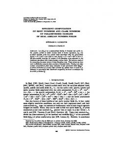
Fig. 1. Local pictures of a regular point and the four types of critical points (minimum, 1-saddle, 2-saddle, and maximum) with shaded oceans, white continents and integral lines [17].
proach similar to the watershed transform [24, 1]. The initial growing of 3-manifolds produces a similar segmentation, however, our algorithm also computes the connectivity of the full Morse-Smale complex, which is necessary for full topology-based simplification of volumetric data. 1.2 Contributions We introduce a new algorithm for computing the Morse-Smale complex for volumetric domains. Cells of all dimensions in the MorseSmale complex are explicitly computed resulting in a partition of the domain. Our algorithm operates on a tetrahedralization, however it uses a point based representation to store cells of the Morse-Smale complex. Given a volumetric scalar field over a grid, we create an implicit tetrahedralization, and find the Morse-Smale complex of the resulting piecewise-linear function. Gyulassy et al. [17] showed how the Morse-Smale complex could be used in visualization and topology-based simplification. We reproduce those results, and show that the algorithm introduced in this paper is faster and more efficient. 2 BACKGROUND Morse theory has been well studied in the context of smooth scalar functions. However, scientific data is often presented as a set of discrete samples over a domain, such as a volumetric grid or a tetrahedralization. We utilize a description of Morse theory for piecewise linear (PL) 3-manifolds presented in Edelsbrunner et al. [10], and apply it to our point-set representation. 2.1 Morse Functions and Morse-Smale Complex A real-valued smooth map f : M → R defined over a compact 3manifold M is a Morse function if all its critical points are nondegenerate (i.e., the Hessian matrix is non-singular for all critical points) and no two critical points have the same function value. Figure 1 shows local neighborhoods of the four types of non-degenerate critical points. An integral line of f is a maximal path in M whose tangent vectors agree with the gradient of f at every point of the path. Each integral line has a natural origin and destination at critical points of f where the gradient becomes zero. Ascending and descending manifolds are obtained as clusters of integral lines having common origin and destination respectively. The Morse-Smale complex partitions M into regions by clustering integral lines that share common origin and destination. In Morse-Smale functions, the integral lines connect critical points of different indices. For example, the 3D cells of the Morse-Smale complex cluster integral lines that originate at a given minimum and terminate at an associated maximum. The cells of different dimensions are called crystals, quads, arcs, and nodes. Note that the Morse-Smale complex is an overlay of ascending and descending manifolds, which individually partition M as well. The arcs form a pairing of critical points that we call the combinatorial structure of the Morse-Smale complex. Figure 2 illustrates that each critical point in the complex is associated with an ascending manifold of dimension 3−index(p) and a descending manifold of dimension index(p), where the index of a minimum, 1-saddle, 2-saddle, and maximum is 0, 1, 2, and 3 respectively. We refer to ascending and descending manifold in general as n-manifolds, where n can be 0,1,2, or 3. 2.2 Piecewise Linear (PL) Functions Scientific data is usually available as a set of discrete samples over a smooth manifold M, represented by a triangulation K. Let K be a triangulation of the given 3-manifold M. The underlying space of K is
Fig. 2. The dimension of ascending (red) and descending (blue) manifolds depends on the index of the corresponding critical points. The ascending manifolds of a minimum, 1-saddle, 2-saddle, and maximum are a volume, a surface, pair of arcs, and a point respectively. Similarly, the descending manifolds are a point, a pair of arcs, a surface, and a volume.
homeomorphic to M. K consists of simplices of dimension 0, 1, 2, and 3, which we refer to as vertices, edges, triangles, and tetrahedra. We denote Ki ⊂ K as the set of i-dimensional simplices in the triangulation, for example, K0 is the set of all vertices. In general, the function defined over K is not a Morse function. We simulate a perturbation [8, Section 1.4] to ensure that all critical points are non-degenerate and hence identify the given distance field as a Morse function. We define some key terms relevant to PL functions: • LINK The set of vertices in the spherical neighborhood of a vertex p ∈ K0 is called the link of p, denoted Lk p • LOWER LINK The lower link of a vertex p ∈ K0 denoted Lk− p is defined as the set of vertices q ∈ K such that q ∈ Lk p and f (q) < f (p). • INCIDENT A set of vertices S ⊆ K0 is incident on a vertex p ∈ K0 if there exists a point q ∈ S such that q ∈ Lk p, i.e. the intersection of S and Lk p is non-empty. We define a quasi Morse-Smale complex for a PL function as a segmentation of K where each n-manifold is made up of simplices in K. The Morse-Smale complex partitions M into regions by clustering integral lines that share common origin and destination. A result of this segmentation is that a n-manifold forms the boundary between n + 1manifold regions. In fact, a critical point of the complex represents exactly the intersection of an ascending and descending manifold. Traditionally, critical points in PL functions are identified by counting the number of lower and higher components in the link of each vertex [9], however, the intersections of ascending and descending manifolds are an equivalent condition for classification: a minimum is the intersection of an ascending 3-manifold and a descending 0-manifold; a 1saddle is the intersection of an ascending 2-manifold and descending 1-manifold; a 2-saddle is the intersection of an ascending 1-manifold and descending 2-manifold; and a maximum is the intersection of an ascending 0-manifold and descending 3-manifold. Let An be an ascending n-manifold, and Dn be a descending n-manifold. Since all n-manifolds are made up of simplices in K, we can represent each nmanifold as the set of vertices that define its simplices. For example, a tetrahedra in an ascending 3-manifold contributes its four corner vertices to the set Ai3 , the ascending 3-manifold with origin i. 2.3 Persistence-based Simplification A function f is simplified by repeated cancellation of its critical points. Canceling a pair of critical points in the Morse-Smale complex represents smoothing the function by modifying gradient behavior in the neighborhood of the critical points. We consider critical point pairs that are connected by an arc in the complex, i.e., they are paired in the combinatorial structure. Therefore, critical point pairs that can be canceled have consecutive indices. The valid cancellations are those of
minimum-1-saddle, 1-saddle-2-saddle, and 2-saddle-maximum pairs. We refer to Gyulassy et al. [17] for a complete characterization of these cancellations. The saddle-extremum and saddle-saddle cancellations can be modeled as the union of manifold regions. In each cancellation, the ascending and descending manifolds of the two critical points are merged across their respective boundaries. For example, in a minimum-1-saddle cancellation, the ascending 3-manifold of the minimum is merged across the ascending 2-manifold of the 1-saddle, and the descending 1-manifold of the 1-saddle is merged with all 1manifolds incident on the descending 0-manifold of the minimum. In a 1-saddle-2-saddle cancellation, the ascending 2-manifold of the 1saddle is merged with all ascending 2-manifolds incident on the ascending 1-manifold of the 2-saddle, and the descending 2-manifold of the 2-saddle is merged with all descending 2-manifolds incident on the 1-manifold of the 1-saddle. The boundaries of the ascending and descending manifold of each critical point must be updated to reflect the removal of those manifolds. However, this is only a combinatorial change in the complex. The above characterization of cancellations leads to a direct implementation when the manifolds are represented as point sets. Repeated cancellation in order of persistence removes critical point pairs in a manner that preserves important features. The persistence of a pair of critical points that are canceled is equal to the absolute difference in their function values. A LGORITHM Overview We use a single sweep to construct both the combinatorial structure of the complex and the geometric structure of the ascending manifolds. A second sweep uses this segmentation to guide construction of the geometry of the descending manifolds in a manner consistent with the topology identified in the first step. We view the construction of the ascending and descending manifolds as an iteration through dimensions, where the interior of each n-manifold is computed via region growing, and its n − 1-manifold boundaries are recursively computed. We denote the interior of an n-manifold Mni as Int(Mni ), and the boundary as Bd(Mni ). Figure 3 shows how we iterate through dimensions while constructing the ascending manifolds.
[a]
[b]
[c]
[d]
3
3.1 Ascending 3-manifolds Given a function f defined over the triangulation K of a volumetric domain, we identify the set of minima Min of the PL function as p ∈ Min ⇐⇒ p ∈ K0 , f (p) < f (q) for all q ∈ Lk p. The set Min contains the “seed points” for the ascending 3-manifolds of f ; each minimum m ∈ Min is the origin for a set of vertices that represent an ascending 3-manifold. We sweep through the domain in sorted order to classify each vertex as interior to an ascending 3-manifold, or lying on the boundary. At each vertex p, we determine whether it is interior or boundary to the ascending 3-manifold Ai3 by inspecting the connected components of the set IntLk− (p, A3 ) = Lk− p ∩ Int(A3 ), the set of vertices already classified as interior to some ascending 3manifold A3 and also in the lower link of p. All vertices q ∈ Lk− p are guaranteed to be classified previously, since we process the vertices in sorted order. If the number n of connected components of IntLk− (p, A3 ) is exactly one, then p is classified as an interior vertex. If n is more than one, then p is classified as part of the boundary between ascending 3-manifolds. Figure 4 shows how we classify a vertex based on its link. Due to the triangulation, it is possible for n to be zero, namely that no vertices in the link of p are interior vertices. This case can happen where boundaries entirely encircle a region, and we resolve it by creating a new ascending 3-manifold originating at p to maintain the combinatorial structure of the complex. 3.2 Ascending 2-manifolds In the first step of the algorithm we found all minima and associated ascending 3-manifolds of f . The vertices classified as boundary form the separating surfaces between the 3-manifold regions. We create ascending 2-manifolds that separate adjacent ascending 3-manifolds. j Two ascending 3-manifolds, Ai3 , and A3 are considered adjacent if they satisfy one of two conditions:
[e] Fig. 3. (a) The algorithm at each iteration identifies interior and boundary vertices of an ascending n-manifold. (b) Using minima as seed points, we grow ascending 3-manifolds, finding vertices that are interior (blue) to a single 3-manifold. The grey region depicts the boundary between ascending 3-manifolds. (c) We next compute ascending 2-manifolds by first identifying interior points. An ascending 2-manifold (green) separates exactly two ascending 3-manifolds. (d) Ascending 1manifolds (yellow) separate a unique set of ascending 2-manifolds. (e) Finally, the maxima (red) are found as the separating sets between ascending 1-manifolds.
1. There exists a boundary vertex p ∈ K0 such that the link of p contains at least one vertex interior to Ai3 , at least one vertex j interior to A3 , and no vertices interior to any other ascending 3manifold. j
2. There exists pi , p j , and pk such that Ai3 and A3 are incident on each, and (pi , p j , pk ) ∈ K2 is a face in the triangulation K. Figure 5 illustrates these rules for determining when two ascending 3-manifolds are adjacent. We create an ascending 2-manifold for every pair of adjacent asij cending 3-manifolds. An ascending 2-manifold A2 separating Ai3 and j A3 consists of all vertices p ∈ K0 such that p is classified as a boundary j and Ai3 and A3 are incident on p. The triangulation of the surface repij resented by A2 is recovered by identifying triangles in K where every ij vertex of the triangle is in A2 . These ascending 2-manifolds represent the combinatorial pairing of minima with 1-saddles in the Morse-Smale complex; each ascending 2-manifold is assigned a 1-saddle, and that saddle is paired with exactly the two minima whose ascending 3-manifolds are separated by the 2-manifold. In this way, we avoid the problem of explicity splitting degenerate multi-saddles; all saddles identified in this way are guaranteed to be simple. We discuss further how multi-saddles are resolved
C C
D p
p
B
p
A
A B
(b)
(a)
(c)
Fig. 4. (a) The lower link (blue points) is connected and classified as interior, therefore the vertex p is an interior vertex. (b) The lower link has multiple regions, therefore p is a boundary vertex. (c) The lower link consisting of the blue and pink vertices is split by the pink vertices, which are classified as boundary, therefore p is classified as a boundary vertex.
B
B b
Fig. 6. Left: Four ascending 2-manifolds A, B, C, and D come together along an ascending 1-manifold. The grey points represent A1 associated with A, B, C, and D, which also happen to separate interior points marked in blue. Right: The boundary between ascending 2-manifolds does not necessarily form a line in the triangulation. Here, the grey points separate A, B, and C, and represent the ascending 1-manifold associated with A, B, and C.
C
S
p a
C A
A
D B
Fig. 5. Left: The vertices in S separate two ascending 3-manifolds A and B. Each vertex in S may additionally separate other ascending 3manifolds. Since the vertices form a face in the triangulation, SAB is an ascending 2-manifold of the complex. Right: A single point p separates the ascending 3-manifolds A and B. However, since no other ascending 3-manifold is incident on p, p forms the ascending 2-manifold SAB of the complex.
in section 4. We identify the adjacency of ascending 2-manifolds in a similar way to identifying the adjacency of ascending 3-manifolds. We first find vertices that are considered interior to an ascending 2-manifold. ij A vertex p ∈ K0 ∩ A2 is interior to an ascending 2-manifold A2 if Ai3 j and A3 are the only interior regions incident on p, and all vertices ij q ∈ Lk p ∩ A2 are also in A2 . Therefore, vertices in A2 that separate exactly two interior regions and do not lie directly on the merging of two 2-manifolds are considered interior to an ascending 2-manifold. The set of vertices that form the boundaries between ascending 2manifolds form a lattice we denote M1 . 3.3 Ascending 1-manifolds The pairing between ascending 3-manifolds and 2-manifolds form the Minima - 1-Saddle connections in the Morse-Smale complex. Similar to finding these connections, we identify pairings between 2-Saddles and 1-Saddles as the pairing of ascending 1-manifolds and the ascending 2-manifolds they separate. A single 1-manifold may form the shared boundary of several ascending 2-manifolds, therefore we associate such an ascending 1-manifold A1 with an n-tuple of 2-manifolds (A02 , . . . , An2 ). A set of ascending 2-manifolds (A02 , . . . , An2 ) are considered adjacent if there exist vertices pi and p j such that (pi , p j ) ∈ K1 is an edge in the triangulation K, and A02 , . . . , An2 are incident on both vertices. An ascending 1-manifold A1 is part of the Morse-Smale complex if and only if (A02 , . . . , An2 ) are adjacent at both vertex endpoints of an edge in K1 and there is no ascending 2-manifold Ai2 such that the ascending 2-manifolds of the set (A02 , . . . , An2 , Ai2 ) are adjacent along both vertex endpoints of an edge in K1 . Therefore, we create an ascending 1-manifold every place where ascending 2-manifolds merge, and that 1-manifold separates all 2-manifolds that are incident along its entire length. Figure 6 shows how we segment M1 to form the ascending 1-manifolds. A vertex p of an ascending 1-manifold A1 is an interior vertex if for all vertices q ∈ Lk p ∩ M1 , A02 , . . . , An2 are incident on q. This condition is true when there are no other ascending 1-manifolds
E
A
Fig. 7. The interior (colored) points of ascending 1-manifolds A, B, C, D, and E meet at a cluster of vertices (grey). This set denotes a maximum node in the complex, since it forms the boundary between the ascending 1-manifolds. The selection of the maximum vertex within A0 associated with A, B, C, D, and E does not change the topology of the complex. We pick the highest vertex in the cluster for which all the ascending 1-manifolds are incident.
in the link of p. The boundaries between ascending 1-manifolds form small disjoint clusters of vertices we denote A0 . Figure 7 shows that a cluster of points can be the boundary between ascending 1-manifolds. 3.4 Maxima Combinatorially, the ascending 1-manifolds incident on each cluster of points in M0 represent the 2-Saddles that are connected to the Maximum represented by the cluster. Maxima can form the boundary between several ascending 1-manifolds, therefore we denote a maximum as A0 associated with an n-tuple of incident ascending 1-manifolds (A01 , . . . , AN 1 ) . Similar to the way we defined ascending 1-manifolds, A0 is a maximum of the Morse-Smale complex if (A01 , . . . , AN 1 ) are adi jacent, and there is no Ai1 such that (A01 , . . . , AN 1 , A1 ) are adjacent. This selects the vertex in each cluster of vertices that is connected to the incident ascending 1-manifolds by an edge in the triangulation K. Figure 7 illustrates that a cluster of vertices are identified as a maximum node in the Morse-Smale complex. 3.5 Descending Manifolds The computation of the ascending manifolds identifies, partially, the combinatorial structure of the Morse-Smale complex and produces a point-set representation of ascending manifolds. We use this structure to guide the construction of the descending manifolds in a manner that incorporates the geometry of the ascending manifolds. The combinatorial structure of the Morse-Smale complex must be maintained: intersections between ascending and descending manifolds must be transversal. We accomplish this explicitly by finding the descending manifold regions restricted to the interior of each ascending n-
[a] [b]
[a]
[b] Fig. 8. (a) The pair of maxima separated by a single edge in the triangulation form an ascending 1-manifold. According to the combinatorial nature of the complex, there must be some vertex in the ascending 1manifold that is a 2-saddle separating the maxima. (b) We resolve this by inserting a vertex into the triangulation at each endpoint of the ascending 1-manifold.
manifold. We find the descending manifold in the interior of an ascending n-manifold to ensure that any classification performed will not affect neighboring ascending n-manifolds. Due to the simulation of differentiability, where integral lines are restricted to lie on edges of the triangulation, it is possible for an ascending n-manifold to have no interior points, or not have enough points to allow the propagation of the descending manifolds. Figure 8 shows such a case, where an ascending 1-manifold consists of exactly one edge in the triangulation. According to the combinatorial structure of the complex, there must be a 2-saddle on this ascending 1-manifold, however, all its vertices are already classified as maxima. One solution is the splitting of tetrahedra by inserting new vertices into the triangulation to ensure interior points are present. Since we represent the Morse-Smale complex as point sets, this splitting corresponds to adding a vertex and symbolic links. We insert a copy of vertices in the boundary of ascending nmanifolds, as shown in Figure 9, in a way that simulates splitting of simplices in the triangulation. We simply duplicate these “split” vertices, without actually splitting tetrahedra. The addition of vertices ensures the presence of the necessary interior vertices for identification of descending manifolds. We use the same region growing to find the descending manifolds within each augmented ascending manifold. We start with ascending 1-manifolds, and classify each interior point as interior/boundary to the descending 3-manifold originating at the maxima that are the endpoints of the ascending 1-manifold. Next we perform the region growing in the interior of each ascending 2-manifold, starting with the classification attained in the first step for its ascending 1-manifold boundaries, and classify each vertex as interior/boundary to the descending 3-manifolds originating at the corners of the ascending 2-manifold. The boundary vertices of the descending 3-manifolds restricted to the ascending 2-manifolds are then identified as interior/boundary to the descending 2-manifolds originating at the 2-saddles found in the first step. The interior points of these descending 2-manifolds restricted to the ascending 2-manifolds form the 1-manifold connector between 1-saddles and 2-saddles. Finally, we perform the full region growing algorithm on each ascending 3-manifold, using the classification of its boundaries from the previous step. 4
D ISCUSSION
The algorithm we present computes a Morse-Smale complex for a perturbed function f p that differs from the Morse-Smale complex of the original function f in several ways. In f p we assume that any two ascending 3-manifolds that are adjacent, i.e. they are sep-
[c] Fig. 9. (a) Three ascending 2-manifolds (green) separated by three ascending 1-manifolds (yellow), which are incident on a maximum (red). (b) First, we insert a copy of the boundary vertex to each ascending 1-manifold, by splitting the edge incident on the maximum. (c) Next, we add a copy of the 1-manifold boundaries to each of the ascending 2-manifolds, further splitting the triangulation. Now, we are guaranteed to have sufficient interior vertices in the ascending manifolds to allow independent identification of descending manifolds.
arated by exactly one vertex in the triangulation, have an ascending 2-manifold separating them. This generates a 1-saddle on the ascending 2-manifold that separates the two minima that are the origins of the ascending 3-manifolds. However, it is possible that in f no such 1saddle exists; the interface between the two ascending 3-manifolds is monotonic. In this case, another pair of ascending 2-manifolds in the Morse-Smale complex of f would merge and separate the ascending 3manifolds, therefore there would be no ascending 2-manifold directly separating the two ascending 3-manifolds. The 1-saddle implied in f p corresponds to perturbing f along the merge of every pair of ascending 2-manifolds, so that each 2-manifold vertex separates exactly those regions that are adjacent to it. Figure 10 illustrates the difference between the complex of f p and the complex of f . The additional critical points inserted, however, have zero persistence, and therefore will be canceled first. In fact, after canceling all zero persistence critical point pairs, the complex of f p will be exactly the same as the complex of f . After the zero persitence critical point pairs are cancelled, we get the same topology for the complex as the algorithm in [17]. The differences between the results are a result of the implicit triangulation we use in this approach, whereas in [17] operates on a piecewise constant hexahedral grid. Our new approach produces geometrically different results depending on whether we construct ascending or descending manifolds first. After all zero persistence pairs are removed, the combinatorial structure of the complexes computed using either ordering will be equivalent. However, some small changes to the geometry of the complex occurr, as the location of saddles might be shifted. Large-scale features, represented by high persistence pairs, are preserved. Our approach to constructing Morse-Smale complexes implicitly handles multi-saddles. We use the link conditions to identify only the minima; all other critical points are classified by the algorithm, thereby simulating differentiability at each vertex, and intrinsically splitting multi-saddles. Each pair of adjacent ascending 3-manifolds is assigned a separating ascending 2-manifold and a 1-saddle, removing the possibility of multi-1-saddles. Similarly, each ascending 1-manifold terminates at a maximum at either end, enforcing the condition that nondegenerate two saddles are connected to exactly two maxima. The
C
C B
A
B
A
Fig. 10. Three ascending 3-manifolds A, B, and C touch in f (left). In the Morse-Smale complex of f there is no 1-saddle separating A and B, therefore the ascending 2-manifold that separates A and C and the ascending 2-manifold that separates B and C merge to separate A and B. The function f p however ensures that there is a 1-saddle between each adjacent ascending 3-manifolds (right). The Morse-Smale complex for f p contains additional critical points, but the persistence pairs introduced, such as the circled 1-saddle - 2-saddle pair, have zero persistence. Canceling all the zero persistence pairs will produce the same configuration as on the left.
construction of f p automatically splits manifolds that would represent a multi-saddle. There are many ways to resolve multi-saddles, and our algorithm produces a complex that corresponds to splitting a multi-saddle with n lower regions into n 1-saddles and a 2-saddle in the middle. 5 5.1
I MPLEMENTATION Data Structures
We implement the algorithm for volumetric data using point sets to represent the ascending/descending manifolds. Each ascending nmanifold contains the set of vertex indices representing the geometric location of its interior vertices, a list of its ascending n − 1-manifold boundaries, and a list of the ascending n + 1-manifolds that contain it in its boundary. These lists represent the combinatorial structure of the complex, since they connect ascending manifolds that originate at critical points differing in index by one. Each ascending manifold also contains a link to the descending manifold that originates at the associated critical point. The descending manifolds contain the set of vertices representing its interior vertices, and a link to the ascending manifold associated with its critical point. The Morse-Smale complex is stored as a list of ascending 0-manifolds, 1-manifolds, 2-manifolds, and 3-manifolds. Storing the set of interior vertices for a 3-manifold region is inefficient. We utilize the fact that the interior vertices of ascending 3-manifolds are contiguous, and store only a single seed vertex from which we can flood-fill the entire ascending 3-manifold region. Descending 3-manifolds are treaded similarly, with the exception that vertices that were symbolically split from its boundary are represented explicitly. This duplicates the storage of the boundary vertices, since they will be present in several descending 3-manifolds. However, this is necessary to be able to maintain a independent classification for the same vertex for each ascending manifold it is contained in. To flood fill a 3-manifold, we store a one byte representation of the classification at each vertex in the dataset. During construction of the complex, it is necessary to query a vertex to determine its classification, and we use this same structure to resolve those queries. Finally, it is necessary to determine at each vertex which ascending manifold it is contained in. We use a hash table to map the index location to the ascending manifold that contains it. The exception to this is the interior vertices of 3-manifolds, where we can determine the ascending 3-manifold by finding the seed point. Just as in [17], we represent cancellation of critical point pairs as a merge tree, merging the interior points of each ascending/descending manifold. To recover the geometry of a particular manifold, we traverse the merge tree and find all leaf nodes that have been merged to form that manifold. The same cancellation operation is performed in each method.
Fig. 12. The maxima (red) identify the locations of the atoms in the potential field of a C4 H4 molecule. The 2-saddles (yellow) separating these maxima represent the bonds between the atoms. A dip in the potential in the center of the molecule is identified by a minimum (blue). 1-saddles are represented as teal spheres.
5.2
Run Time Behavior
Performing the sweep constructing the ascending manifolds requires a classification operation at each vertex in the dataset, which is dependent on the size k of the link in the triangulation K. While it is possible for a triangulation to have k be on the order of the number of vertices of the dataset, in practice it is bounded by a constant. The points are processed in sorted order. The total running time to construct the ascending manifolds is O(n lg n) where n is the number of vertices in the dataset. In the construction of the descending manifolds new vertices are inserted into the triangulation. The number of vertices is dependent on the geometric size and distribution of features in the dataset, and the size of the Morse-Smale complex. In the worst case, where every other vertex is a maximum, each vertex must be split into k3 new vertices. Practically, however, the number of split vertices is a small fraction of n, and is still bounded by a constant, therefore the expected running time is still O(n lg n). Cancellations are performed at interactive speeds, since we simply add nodes to a merge tree for each cancellation. The geometry of the sets of vertices representing the ascending/descending manifolds do not change. In fact, the basic operations are the same as presented by Gyulassy et al. [17], where we simply replace the geometry component of each node in the complex with a point set. 6
R ESULTS
The input data is given as scalar samples on a three-dimensional regular hexahedral grid. We create a triangulation of this function by defining vertices to lie at sample locations, and the tetrahedralization given by some implicit connectivity between the vertices. In general, our method works for any tetrahedralized data, regular or irregular. In our examples, our implicit connectivity subdivides each voxel of the original data into six tetrahedra, in a manner where each vertex is connected in a consistent manner to its neighbors. This consistency is a valuable optimization when searching for regions in the link of a vertex, since we can use the same graph to represent the link of any vertex, and just replace the values at the nodes of the graph. We construct the ascending and descending manifolds to obtain the Morse-Smale complex of a permuted representation of the function, and then construct the Morse-Smale complex of the actual function by canceling all zero persistence critical point pairs. In the example in Figure 12, we show how the Morse-Smale complex can be used to identify the locations of the atoms in the C4 H4 molecule. Figure 11 illustrates the use of our algorithm in finding the features for some well known datasets. Table 1 shows the timing information for these datasets, as well as a comparison in terms of running time to the construction using an artificial complex [17]. A direct comparison between the algorithm reveals that the method we introduce in this paper is much faster for computing the initial full resolution complex. Instead of performing costly cancellation opera-
[a]
[c]
[e]
[b]
[d]
[f]
Fig. 11. The Morse Smale complex computed for three well-known datasets. The neghip data set (a) is a result of a spatial probability distribution of the electrons in a high-potential protein molecule. Overlaying the 2-saddle-maximum arcs of the simplified complex (b) shows the structure of high-potential regions. The hydrogen data (c) is a result of a simulation of the spatial probability distribution of the electron in a hydrogen atom residing in a strong magnetic field. We extract the same features (d) for this dataset as in [17]. The aneurism data (e), is a Rotational C-arm x-ray scan of the arteries of the right half of a human head. The 2-saddle-maximum arcs of the simplified complex (f) trace out structure of the arteries.
Data set Neghip Hydrogen Aneurism
Size 64 × 64 × 64 128 × 128 × 128 256 × 256 × 256
(a) 7s 27s 3m 51s
(b) 2m 35s 45m ∞
members of the Visualization and Computer Graphics Research Group at the Institute for Data Analysis and Visualization (IDAV) at the University of California, Davis. R EFERENCES
Table 1. The finest resolution Morse-Smale complex is computed for well known datasets. We compare the running time of our algorithm (a) to the simplification based algorithm presented in [17] (b).
tions within each voxel, our region growing skips through the monotonic volumes in the data, and only requires special analysis at the boundaries of 3-manifolds. This leads to a much more efficient algorithm. Even though our point-set based method was implemented without sophisticated optimizations, we avoid having to store an artificial complex, and therefore the memory footprint is up to 10 times smaller. 7
C ONCLUSIONS
We have presented an efficient algorithm for computing the MorseSmale complex for volumetric domains. We have shown that our algorithm is faster and more efficient than previous methods. The region growing algorithm we present computes all dimensional components of the complex, which has several advantages. The complete decomposition of space allows us to consider topology-based smoothing, compression, and improved topology-based visualization. The point-set based method applies to general tetrahedralized meshes, while maintaining speed and robustness on gridded data. ACKNOWLEDGEMENTS Attila Gyulassy is supported by a Student Employee Graduate Research Fellowship (SEGRF), Lawrence Livermore National Laboratory. This work was also supported in part by the National Science Foundation under contract ACI 9624034 (CAREER Award), and a large Information Technology Research (ITR) grant. We thank the
[1] S. Beucher. Watershed, heirarchical segmentation and waterfall algorithm. In J. Serra and P. Soille, editors, Mathematical Morphology and its Applications to Image Processing, pages 69–76, 1994. [2] P.-T. Bremer, H. Edelsbrunner, B. Hamann, and V. Pascucci. A topological hierarchy for functions on triangulated surfaces. IEEE Transactions on Visualization and Computer Graphics, 10(4):385–396, 2004. [3] H. Carr, J. Snoeyink, and U. Axen. Computing contour trees in all dimensions. In Symposium on Discrete Algorithms, pages 918–926, 2000. [4] H. Carr, J. Snoeyink, and M. van de Panne. Simplifying flexible isosurfaces using local geometric measures. In Proc. IEEE Conf. Visualization, pages 497–504, 2004. [5] A. Cayley. On contour and slope lines. The London, Edinburgh and Dublin Philosophical Magazine and Journal of Science, XVII:264–268, 1859. [6] Y.-J. Chiang and X. Lu. Progressive simplification of tetrahedral meshes preserving all isosurface topologies. Computer Graphics Forum, 22(3):493–504, 2003. [7] P. Cignoni, D. Constanza, C. Montani, C. Rocchini, and R. Scopigno. Simplification of tetrahedral meshes with accurate error evaluation. In Proc. IEEE Conf. Visualization, pages 85–92, 2000. [8] H. Edelsbrunner. Geometry and Topology for Mesh Generation. Cambridge Univ. Press, England, 2001. [9] H. Edelsbrunner, J. Harer, V. Natarajan, and V. Pascucci. Morse-Smale complexes for piecewise linear 3-manifolds. In Proc. 19th Ann. Sympos. Comput. Geom., pages 361–370, 2003. [10] H. Edelsbrunner, J. Harer, and A. Zomorodian. Hierarchical MorseSmale complexes for piecewise linear 2-manifolds. Discrete and Computational Geometry, 30(1):87–107, 2003. [11] R. Forman. A user’s guide to discrete morse theory, 2001. [12] M. Garland and P. S. Heckbert. Simplifying surfaces with color and texture using quadric error metrics. In Proc. IEEE Conf. Visualization, pages 263–269, 1998.
[13] M. Garland and Y. Zhou. Quadric-based simplification in any dimension. ACM Transactions on Graphics, 24(2):209–239, 2005. [14] T. Gerstner and R. Pajarola. Topology preserving and controlled topology simplifying multiresolution isosurface extraction. In Proc. IEEE Conf. Visualization, pages 259–266, 2000. [15] I. Guskov and Z. Wood. Topological noise removal. In Proc. Graphics Interface, pages 19–26, 2001. [16] A. Gyulassy, V. Natarajan, V. Pascucci, P.-T. Bremer, and B. Hamann. Topology-based simplification for feature extraction from 3d scalar fields. In Proc. IEEE Conf. Visualization, pages 535–542, 2005. [17] A. Gyulassy, V. Natarajan, V. Pascucci, P. T. Bremer, and B. Hamann. A topological approach to simplification of three-dimensional scalar fields. IEEE Transactions on Visualization and Computer Graphics (special issue IEEE Visualization 2005), pages 474–484, 2006. [18] H. Hoppe. Progressive meshes. In Proc. SIGGRAPH, pages 99–108, 1996. [19] T. Lewiner, H. Lopes, and G. Tavares. Applications of forman’s discrete morse theory to topology visualization and mesh compression. IEEE Transactions on Visualization and Computer Graphics, 10(5):499–508, 2004. [20] J. C. Maxwell. On hills and dales. The London, Edinburgh and Dublin Philosophical Magazine and Journal of Science, XL:421–427, 1870. [21] V. Natarajan and H. Edelsbrunner. Simplification of three-dimensional density maps. IEEE Transactions on Visualization and Computer Graphics, 10(5):587–597, 2004. [22] S. Rana. Topological Data Structures for Surfaces: An Introduction to Geographical Information Science. Wiley, 2004. [23] G. Reeb. Sur les points singuliers d’une forme de Pfaff compl`etement int´egrable ou d’une fonction num´erique. Comptes Rendus de L’Acad´emie ses S´eances, Paris, 222:847–849, 1946. [24] J. Roerdink and A. Meijster. The watershed transform: Definitions, algorithms and parallelization techniques, 1999. [25] S. Smale. Generalized Poincar´e’s conjecture in dimensions greater than four. Ann. of Math., 74:391–406, 1961. [26] S. Smale. On gradient dynamical systems. Ann. of Math., 74:199–206, 1961. [27] O. G. Staadt and M. H. Gross. Progressive tetrahedralizations. In Proc. IEEE Conf. Visualization, pages 397–402, 1998. [28] S. Takahashi, G. M. Nielson, Y. Takeshima, and I. Fujishiro. Topological volume skeletonization using adaptive tetrahedralization. In Proc. Geometric Modeling and Processing, pages 227–236, 2004. [29] S. Takahashi, Y. Takeshima, and I. Fujishiro. Topological volume skeletonization and its application to transfer function design. Graphical Models, 66(1):24–49, 2004. [30] Z. Wood, H. Hoppe, M. Desbrun, and P. Schr¨oder. Removing excess topology from isosurfaces. ACM Transactions on Graphics, 23(2):190– 208, 2004.