Efficient Computation of Robust Low-Rank Matrix ... - Semantic Scholar

Efficient Computation of Robust Low-Rank Matrix Approximations in the Presence of Missing Data using the L1 Norm Anders Eriksson and Anton van den Hengel School of Computer Science University of Adelaide, Australia {anders.eriksson, anton.vandenhengel}@adelaide.edu.au

Abstract The calculation of a low-rank approximation of a matrix is a fundamental operation in many computer vision applications. The workhorse of this class of problems has long been the Singular Value Decomposition. However, in the presence of missing data and outliers this method is not applicable, and unfortunately, this is often the case in practice. In this paper we present a method for calculating the low-rank factorization of a matrix which minimizes the L1 norm in the presence of missing data. Our approach represents a generalization the Wiberg algorithm of one of the more convincing methods for factorization under the L2 norm. By utilizing the differentiability of linear programs, we can extend the underlying ideas behind this approach to include this class of L1 problems as well. We show that the proposed algorithm can be efficiently implemented using existing optimization software. We also provide preliminary experiments on synthetic as well as real world data with very convincing results.

1. Introduction This paper paper deals with low-rank matrix approximations in the presence of missing data. That is, the following optimization problem ˆ (Y − U V ) ||, min ||W U,V

(1)

where Y ∈ Rm×n is a matrix containing some measurements, and the unknowns are U ∈ Rm×r and V ∈ ˆ ∈ Rr×n .We let w ˆij represent an element of the matrix W Rm×n such that w ˆij is 1 if yij is known, and 0 otherwise. Here || · || can in general be any matrix norm, but in this work we consider the 1-norm, X ||A||1 = |aij |, (2) i,j

978-1-4244-6983-3/10/$26.00 ©2010 IEEE

in particular. The calculation of a low-rank factorization of a matrix is a fundamental operation in many computer vision applications. It has been used in a wide range of problems including structure-from-motion[18], polyhedral object modeling from range images[17], layer extraction[12], recognition[19] and shape from varying illumination[11]. In the case where all of the elements of Y are known the singular value decomposition may be used to calculate the best approximation as measured by the L2 norm. It is often the case in practice, however, that some of the elements of Y are unknown. It is also common that the noise in the elements of Y is such that the L2 norm is not the most appropriate. The L1 norm is often used to reduce sensitivity to the presence of outliers in the data. Unfortunately, it turns out that introducing missing data and using the L1 norm instead, makes the problem (1) significantly more difficult. It is firstly a non-smooth problem, so many of the standard optimization tools available will not be applicable. Secondly, it is a non-convex problem so certificates of global optimality are in general hard to provide. And finally it can also be very computationally demanding task to solve, when applied to a real world applications the number of unknowns are typically very large. In this paper we will present a method that efficiently computes a low rank approximation of a matrix in the presence of missing data, under the L1 norm, by effectively addressing the issues of non-smoothness and computational requirements. Our proposed method should be viewed as a generalization of, one of the more successful algorithms for the L2 case, the Wiberg method [20].

1.1. Notation All of the variables used in this paper are either clearly defined or should otherwise be obvious from the context in which they appear. Additionally, In denotes a n × n identity matrix, and ⊗ are the Hadamard and Kronecker products respectively. Upper case roman letters denote matrices

and lower case ones, vectors and scalars. We also use the convention that v = vec(V ), a notation that will be used interchangeably throughout the remainder of this paper.

2. Previous Work The subject of matrix approximation has been extensively studied, especially using L2 type norms. A number of different names for the process are used in the literature, such as principal component analysis, subspace learning and matrix or subspace factorization. In this paper we describe the problem in terms of the search for a pair of matrices specifying a low rank approximation of a measurement matrix, but the approach is equally applicable to any of these equivalent problems. For an outstanding survey of many of the existing methods for least L2 -norm factorization see the work of [5]. This paper also contains a direct quantitative comparison of a number of key methods. Unfortunately, their comparison did not include the Wiberg algorithm [20]. This method, which was first proposed more than 30 years ago, has been largely misunderstood or neglected by computer vision researchers. An issue which was addressed in the excellent work of [16], effectively reintroducing the Wiberg algorithm to the vision community. It was also shown there, that on many problems the Wiberg method outperforms many of the existing, more recent methods. The subject of robust matrix factorization has not received as much attention within computer vision as it has in other areas (see [1, 15] for example). This is beginning to be addressed, however. A very good starting point towards a study of more robust methods, however, is the work of [9]. One of the first methods suggested was Iteratively Re-weighted Least Squares which minimizes a weighted L2 norm. The method is unfortunately very sensitive to initialization (see [13] for more detail). Black and Jepson in [4] describe a method by which it is possible to robustly recover the coefficients of a linear combination of known basis vectors that best reconstructs a particular input measurement. This might be seen as a robust method for the recovery of V given U in our context. De la Torre and Black in [9], present a robust approach to Principal Component Analysis which is capable of recovering both the basis vectors and coefficients, which is based on the Huber distance. The L1 norm was suggested by Croux and Filzmoser in [7] as a method for addressing the sensitivity of the L2 norm to outliers in the data. The approach they proposed was based on a weighting scheme which applies only at the level of rows and columns of the measurement matrix. This means that if an element of the measurement matrix is to be identified as an outlier then its entire row or column must also be so identified. Ke and Kanade in [13] present a factorization method

based on the L1 norm which does not suffer from the limitations of the Croux and Filzmoser approach and which is achieved through alternating convex programs. This approach is based on the observation that, under the L1 -norm, for a fixed U , the problem (1) can be written as a linear problem in V , and vice versa. A succession of improved matrix approximations can then be obtained by solving a sequence of such linear programs, alternately fixing U and V . It was also shown here, that one can also solve the Huber-norm, an approximation of the L1 -norm, in a similar fashion, with the difference that each subproblem now is a quadratic problem. Both these formulations do result in convex subproblems, for which efficient solvers exist, however this does not guarantee that global optimality is obtained for the original problem in the L1 -norm. The excellent work by [6] also needs mentioning. Here they apply Branch and Bound and convex under estimators to the general problem of bilinear problem, which includes (1), both under L1 and L2 norms. This approach are provably globally optimal, but is in general very time consuming and in practice only useful for small scale problems.

2.1. The Wiberg Algorithm As previously mentioned the Wiberg algorithm is a numerical method developed for the task of low-rank matrix approximation with missing data using the L2 -norm. We will in this section give a brief description of the underlying ideas behind this method in an attempt to motivate some of the steps taken in the derivation of our generalized version to come. The Wiberg algorithm is initially based on the observation that, for a fixed U in, (1)the L2 -norm becomes a linear, least-squares minimization problem in V , min ||W y − W (In ⊗ U )v||22 , v

(3)

W = diag(w), ˆ with a closed-form solution given by (4). v ∗ (U ) = G(U )T G(U )


−1

G(U )W y,

(4)

where G(U ) = (In ⊗ U ). Similar statements can also be made for fixed values of V , min ||W y − W (V T ⊗ Im )u||22 , u
−1 ∗ u (V ) = F (V )T F (V ) F (V )W y,

(5) (6)

and F (V ) = (V T ⊗ Im ). Here it should be mentioned that using (4) and (6), alternatively fixing U while updating V , and vice versa, was one of the earliest algorithms for finding matrix approximations in the presence of missing data. This process is also known as the alternated least squares (ALS) approach. The disadvantage, however, is that it has in practice been shown

to converge very slowly (see [5], for example). The alternated LP and QP approaches of [13] were motivated by this method. Continuing with the Wiberg approach, by substituting (4) into equation (5) we get min ||W y − W U V ∗ (U )||22 = ||W y − φ(U )||22 ,

(7)

U

a non-linear least squares problem in U . It is the application of the Gauss-Newton method [3] to the above problem that results in the Wiberg algorithm. The difference between the Wiberg algorithm and ALS may thus be interpreted as the fact that the former effectively computes Gauss-Newton updates while the latter carries out exact cyclic coordinate minimization. As such, the Wiberg sequence of iterates Uk are generated by approximating φ by its first order Taylor expansion at Uk and solving the resulting subproblem min = ||W y − δ

∂φ(Uk ) 2 δ||2 . ∂U

(8)

If we let Jk denote the Jacobian ∂φ(Uk )/∂U and we can write the solution to (8) as δk∗ = JkT Jk


−1

JkT W y,

(9)

the well known normal equation. The next iterate Uk+1 is then given by Uk+1 = Vk + δk∗ .

3. Linear Programming and Differentiation Before moving on we first need to show some additional properties of linear programming. This section deals with the sensitivity of the solution to a linear program with respect to changes in the coefficients of its constraints. Lets consider a linear program in standard, or canonical form: min

x∈Rn

cT x

s.t. Ax = b x≥0

(10) (11) (12)

Definition 3.1. Given the set of m linear equations in n unknowns, Ax = b, let B be be any nonsingular m × m submatrix made up of columns of A. Then, if all n − m components of x not associated with columns of B are set equal to zero, the solution to the resulting set of equations is said to be a basic solution to (10)-(12) with respect to the basis B. The components associated to with columns of B are called basic variables. Theorem 3.1. Fundamental theorem of Linear Programming Given a linear program in canonical form such as (10)-(12), then if the problem is feasible there always exists an optimal basic solution. Given that a minimizer x∗ of the linear program (10)(12) may been obtained using some optimization algorithm, we are interested in the sensitivity of the minimizer with respect to the coefficients of the constraints. That is, we wish to compute the partial derivatives ∂x∗ /∂A and ∂x∗ /∂b. The following theorem is based on the approach of Freund in [10]. Theorem 3.2. Let B be a unique optimal basis h ∗ ifor (10)x (12) with minimizer x∗ partitioned as x∗ = x∗B . Where N x∗B is the optimal basic solution and x∗N = 0 the optimal non-basic solution. Reordering the columns of A if necessary, there is a partition of A such that A = [B N ], and N are the columns of A associated with the non-basic variables x∗N . Then x∗ is differentiable at A, b with the partial derivatives given by ∂x∗B ∂B ∂x∗B ∂N ∂x∗B ∂b ∂x∗N ∂x∗N = ∂A ∂b

(13)

=

0

(14)

= B −1

(15)

=

(16)

0.

Proof. Given the set of optimal basic variables, the linear program 10 can be written min

xB ∈Rm

with c ∈ Rn , A ∈ Rm×n and b ∈ Rm . It can furthermore be assumed, without loss of generality, that A has full rank. This class of problem has been studied extensively for over a century. As a result there exist a variety of algorithms for efficiently solving (10)-(12). Perhaps the most known well algorithm is the simplex method of [8]. It is the approach taken in that algorithm that we will follow in this section. First, from [14] (pp. 19-21), we have the following definition and theorem.

= −(x∗B )T ⊗ B −1

cTB xB

s.t. BxB = b xB ≥ 0 xN = 0

(17) (18) (19) (20)

where cB ∈ Rm contains the elements of c associated with the basic variables only. Since B is of full rank and we know it is an optimal and feasible basis for (10)-(12) it follows that the solution to BxB = b is both feasible (xB ≥ 0) and optimal. The above statements represent the foundation of the simplex method.

Now, since by assumption, the basis B is unique we have that x∗B = B −1 b x∗N = 0

(21) (22)

and as B is a smooth bijection from Rm onto itself, then x∗ is differentiable with respect to the coefficients in A and b. Differentiation of (13) becomes ∂x∗B ∂B

Unfortunately, this is not a least squares minimization problem so the Gauss-Newton algorithm is not applicable. Nor does v ∗ (U ) have an easily differentiable, closed-form solution, but the results of the previous section allow us to continue in a similar fashion. It can be shown that, by letting v = v + − v − , an equivalent formulation of (30) is  v+ 

min

v + ,v − ,t,s


∂ = ∂B B −1 b
−1 = bT ⊗ Im ∂B
−T∂B −1
T = − b ⊗ Im B ⊗B = −(x∗B )T ⊗ B −1 .

(23) s.t. (24)

In conclusion, by combining the results of theorem 3.1 we can write the derivatives as   ∂x∗ −(x∗B )T ⊗ B −1 0m×(n−m)m (27) = 0(n−m)×m2 0(n−m)×(n−m)m ∂A   ∂x∗ B −1 = . (28) 0(n−m)×m ∂b

4. The L1 -Wiberg Algorithm In this section we will present the derivation of a generalization of the Wiberg algorithm to the L1 -norm. We will follow a similar approach to the derivation of the standard Wiberg algorithm. That is, by rewriting the problem as a function of U only, then linearizing it, solving the resulting subproblem and updating the current iterate using the minimizer of said subproblem. Our starting point for the derivation our generalization of the Wiberg algorithm is again the minimization problem ˆ (Y − U V ) ||1 . min ||W U,V

(29)

Following the approach of section 2.1 we first note that for fixed U and V it is possible to rewrite the optimization problem (29) as v ∗ (U ) = arg min ||W y − W (In ⊗ U )v||1 ,

(30)

u∗ (V ) = arg min ||W y − W (V T ⊗ Im )u||1 ,

(31)

v

u

h |

(25) (26)

Equations (14)-(16) follow trivially from the differentiation of (21) and (22).

both linear problem in V and U respectively. Substituting (30) into equation (31) we obtain

v− t s i  v+ −G(U ) G(U ) −I v− I G(U ) −G(U ) −I t {z } s A(U )

[ 0 0 1T 0 ]

+

(33)  =

h

−W y Wy

i

(34)

| {z } b

−

v , v , t, s ≥ 0 (35) v + , v − ∈ Rrn , t ∈ Rmn , s ∈ R2mn . (36) Note that (33)-(36) here is a linear program in canonical form, allowing us to apply theorem 3.1 directly. Let V ∗ (U ) denote the optimal basic solution of (33)-(36). Assuming that the prerequisites of theorem 3.1 hold, then V ∗ (U ) is differentiable and we can compute the Jacobian of the nonlinear function φ1 (U ) = W U V ∗ (U ). Using (27) and applying the chain-rule, we obtain ∂G ∂U ∂A ∂U ∂v ∂U

(Inr ⊗ W ) (Tr,n ⊗ Im ) (vec(In ) ⊗ Imr )(37) h ∂G ∂G i − ∂U ∂U 0 = 0 (38) ∂G − ∂G 0 =

∂U

= Q

∗ T (vB )

∂U

⊗ B −1




QT ⊗ I2mn


∂A ∂U

(39)

Here Tm,n denotes the mn × mn matrix for which Tm,n vec(A) = vec(AT ), and Q ∈ Rmn×m is obtained by removing the columns corresponding to the non-basic variables of x∗ from the identity matrix Imn . Combining the above expressions we arrive at ∂ ∂v (W U V ∗ (U )) = W G(U ) + ∂U ∂U
∗ T (vB ) ⊗ W (In ⊗ Tr,n ⊗ Im ) (vec(In ) ⊗ Imr ) J(U ) =

(40)

The Gauss-Newton method, in the least squares case, works by linearizing the non-linear part and solving the resulting subproblem. By equation (40) the same can be done for φ1 (U ). Linearizing W y − W U V ∗ (U ) by its first order Taylor expansion results in the following approximation of (32) around Uk f˜(δ) = ||W y − J(Uk )(δ − uk )||1 .

(41)

Minimizing (41)

min f (U ) = ||W y − W U V ∗ (U )||1 = U

= ||W y − φ1 (U )||1 .

(32)

min ||W y − J(U )(δ − u)||1 δ

(42)

is again a linear problem, but now in δ. [ 0 1T ] [ δt ] i h i h ∗ −J(U )−I δ ] = −(W y−W vec(U V )) [ s.t. ∗ t J(U )−I W y−W vec(U V )

min δ,t

||δ||1 ≤ µ δ ∈ Rmr , t ∈ Rmn .

Algorithm 1: L1 -Wiberg Algorithm (43) 1

(44)

3

(45) (46)

Let δk∗ be the minimizer of (43)-(46), with U = Uk , then the update rule for our proposed method is simply Uk+1 = Uk + δk∗ .

2

(47)

Note that in (44) we have added the constraint ||δ||1 ≤ µ. This is done as a trust region strategy to limit the step sizes that can be taken at each iteration so to ensure a nonincreasing sequence of iterates. See algorithm 1 below for details on how the step length µ is handled. We are now ready to present our complete L1 -Wiberg method in Algorithm 1. Proper initialization is a crucial issue for any iterative algorithm and can greatly affect its performance. Obtaining this initialization is highly problem dependent, for certain applications good initial estimates of the solution are readily available and for others finding a sufficiently good U0 might be considerably more demanding. In this work we either initialized our algorithm randomly or through the rankˆ ⊗Y. r truncation of the singular value decomposition of W Finally, a comment on the convergence of the proposed algorithm. We know that, owing to the use of trust region setting, it can be shown that algorithm 1 will produce a sequence of iterates {U0 , ..., Uk } with non-increasing function values, f (U0 ) ≥ ... ≥ f (Uk ) ≥ 0}. We currently have no proof, however, that the assumptions of theorem 3.1 always hold, which is a requirement for the differentiability of V ∗ (U ). Unfortunately this non-smoothness prevents the application of the standard tools for proving convergence to a local minima. In our considerable experimentation, however, we have never observed an instance in which the algorithm does not converge at a local minima.

5. Experiments In this section we present a number of experiments carried out to evaluate our proposed method. These include real and synthetic tests. We have evaluated the performance of the L1 -Wiberg algorithm method against that of two of the state of the art methods presented by Ke and Kanade in [13], (alternated LP and alternated QP). All algorithms were implemented in Matlab. Linear and quadratic optimization subproblems were solved using linprog and quadprog respectively.

4

5 6 7 8 9 10 11 12 13 14 15 16

input : U0 , 1 > η2 > η1 > 0 and c > 1 k=0; repeat Compute the Jacobian of φ1 = J(Uk ) using (37)-(40) ; Solve the subproblem (43)-(46) to obtain δk∗ ; f (Uk ) − f (Uk + δ ∗ ) Let gain = ; f˜(Uk ) − f˜(Uk + δ ∗ ) if gain ≥  then Uk+1 = Uk + δ ∗ ; end if gain < η1 then µ = η1 ||δ ∗ ||1 end if gain > η2 then µ = cµ end k = k + 1; until convergence ; Remarks. • Lines 9-14 are a standard implementation for dealing with µ, the size of the trust region in the subproblem (43)-(46).see for instance [2] for further details. • Typical parameter values used were η1 = 14 , η2 = 43 ,  = 10−3 and c = 2. • In the current implementation we use a simple termination criteria. Iteration is stopped when the reduction in function value f (Uk ) − f (Uk+1 ) is deemed sufficiently small (≤ 10−6 ).

5.1. Synthetic Data The aim of the experiments in this section was to empirically obtain a better understanding of the following properties of each of the tested algorithm, resulting error, rate of convergence, execution time and the computational requirements. For the synthetic tests a set of randomly created measurement matrices were generated. The elements of the measurement matrix Y were drawn from a uniform distribution between [−1, 1]. Then 20% of the elements were chosen at random and designated as missing by setting the correˆ to 0. In addition, to simusponding entry in the matrix W late outliers, uniformly distributed noise over [−5, 5] were added to 10% of the elements in Y . Since the alternated QP method of Ke and Kanade relies on quadratic programing and as such does not scale as

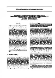
well as linear programs we deliberately kept the synthetic problems relatively small, with m = 7, n = 12 and r = 3. Figure 1 shows a histogram of the error produced by each algorithm on 100 synthetic matrices, created as described above. It can be seen in this figure that our proposed method

Figure 1. A histogram representing the frequency of different magnitudes of error in the estimate generated by each of the methods. [Frequency vs. Error]

clearly outperforms the other two. But what should also be noted here is the poor performance of the alternated linear program approach. Even though it can easily be shown that this algorithm will produce a non-increasing sequence of iterates, there is no guarantee that it will converge to a local minima. This is what we believe is actually occurring in these tests. The alternated linear program converges to a point that is not a local minima, typically after only a small number of iterations. Owing to its poor performance we have excluded this method from the remainder of experiments. Next we examine the convergence rate of the algorithms. A typical instance of the error convergence from from both the AQP and L1 -Wiberg algorithms, applied to one of the synthetic problems, can be seen in figure 2. These figures are not intended to show the quality of the final solution, but rather how it quickly it is obtained by the competing methods. Figure 3 depicts the performance of the algorithms in 100 synthetic tests and is again intended to show convergence rate rather than the final error. Note the independent scaling of each set of results and the fact that the Y-axis is on a logarithmic scale. Again it is obvious that the L1 Wiberg algorithm significantly outperforms the alternated quadratic programming approach. It can be seen that the latter method has a tendency to flatline, that is to converge very slowly after an initial period of more rapid progress. This is a behavior that has also been observed for alternated approaches in the L2 instance, see [5]. Table 1 summarizes the same set of synthetic tests. What should be noted here is the low average error produced by our method, the long execution time of the alternated

Figure 2. Plots showing the norm of the residual at each iteration of two randomly generated tests for both the L1 Wiberg and alternated quadratic programming algorithms. [Residual norm vs. Iteration]

Figure 3. A plot showing the convergence rate of the alternated quadratic programming and L1 -Wiberg algorithms over 100 trials. The error are presented on a logarithmic scale. [Log Error vs. Iteration]

quadratic program approach and the poor results obtained by alternated linear program method. The results of these experiments, although confined to smaller scale problems, do indeed demonstrate the promise of our suggested algorithm.

5.2. Structure from Motion Next we present an experiment on a real world application, namely structure from motion. We use the well known dinosaur sequence, available from http://www.robots.ox.ac.uk/˜vgg/, contain-

Algorithm Error (L1 ) Execution Time (sec) # Iterations # LP/QP solved Time per LP/QP ∗

Alt. LP [13] 4.60 0.16 4.72 9.44 0.016

Alt. QP [13] 2.29 93.57 177.64∗ 355.28∗ 0.264∗

Wiberg L1 (Alg.1) 1.01 1.51 21.77 24.13 0.061

The alternated QP algorithm was terminated after 200 iterations and 400 solved quadratic programs.

Table 1. The averaged results from running 100 synthetic experiments.

ing projections of 319 points tracked over 36 views. Now, finding the full 3D-reconstruction of this scene can be posed as a low-rank matrix approximation task. In addition, as we are considering robust approximation in this work, we also included outliers to the problem by adding uniformly distributed noise [−50, 50] to 10% of the tracked points. We applied our proposed method to this problem, initializing it using truncated singular value decomposition as described in the previous section. For comparison we also include the result from running the standard Wiberg algorithm. Attempts to evaluate the AQP method on this on the same data were abandoned when the execution time exceeded several of hours. The residual for the visible points of the two different matrix approximations is given in figure 4. The L2 norm ap-

of the residual. In the L1 case this does not seem to occur. Instead the reconstruction error is concentrated to a few elements of the residual. The root mean square error of the inliers only, as well as execution times are given in table 2 The resulting reconstructed scene can be seen in figure 5.

6. Conclusion In this paper we have studied the problem of low-rank matrix approximation in the presence of missing data. We have proposed a method for solving this task under the robust L1 norm which can be interpreted as a generalization of the standard Wiberg algorithm. We have also shown through a number of experiments, on both synthetic and real world data, that the L1 Wiberg method proposed is both practical and efficient and performs very well in comparison to other existing methods. Further work in the area will include an investigation into the convergence properties of the algorithm and particularly the search for a mathematical proof that the algorithm indeed converges to a local minima. Jointly, the issue of non-differentiable points of φ1 should also be further investigated.

7. Acknowledgements This research was supported under Australian Research Council’s Discovery Projects funding scheme (project DP0988439).

References

Figure 4. Resulting residuals using the standard Wiberg algorithm (top), and our proposed L1 -Wiberg algorithm (bottom).

proximation seems to be strongly affected by the presence of outliers in the data. The error in the matrix approximation appears to be evenly distributed among all the elements

[1] P. Baldi and K. Hornik. Neural networks and principal component analysis: learning from examples without local minima. Neural Netw., 2(1):53–58, 1989. 2 [2] M. Bazaraa, H. Sherali, and C. Shetty. Nonlinear Programming, Theory and Algorithms. Wiley, 1993. 5 [3] A. Bjorck. Numerical Methods for Least Squares Problems. SIAM, 1995. 3 [4] M. J. Black and A. D. Jepson. Eigentracking: Robust matching and tracking of articulated objects using a view-based representation. In International Journal of Computer Vision, volume 26, pages 329–342, 1998. 2

Algorithm RMS Error of Inliers Execution Time

Alt. QP [13] >4 hrs

Wiberg L2 [20] 2.029 3 min 2 sec

Wiberg L1 (Alg. 1) 0.862 17 min 44 sec

Table 2. Results from the dinosaur sequence with 10% outliers.

Figure 5. Images from the dinosaur sequence, and the resulting reconstruction using our proposed method.

[5] A. M. Buchanan and A. W. Fitzgibbon. Damped newton algorithms for matrix factorization with missing data. In Conference on Computer Vision and Pattern Recognition, volume 2, pages 316–322, 2005. 2, 3, 6 [6] M. K. Chandraker and D. J. Kriegman. Globally optimal bilinear programming for computer vision applications. In Conference on Computer Vision and Pattern Recognition, 2008. 2 [7] C. Croux and P. Filzmoser. Robust factorization of a data matrix. In In COMPSTAT, Proceedings in Computational Statistics, pages 245–249, 1998. 2 [8] G. Dantzig. Linear Programming and Extensions . Princeton University Press, 1998. 3 [9] F. De La Torre and M. J. Black. A framework for robust subspace learning. Int. J. Comput. Vision, 54(1-3):117–142, 2003. 2 [10] R. M. Freund. The sensitivity of a linear program solution to changes in matrix coefficients. Technical report, Massachusetts Institute of Technology, 1984. 3 [11] H. Hayakawa. Photometric stereo under a light source with arbitrary motion. Journal of the Optical Society of America A, 11(11), 1992. 1 [12] Q. Ke and T. Kanade. A subspace approach to layer extraction. Computer Vision and Pattern Recognition, IEEE Computer Society Conference on, 2001. 1 [13] Q. Ke and T. Kanade. Robust L1 norm factorization in the presence of outliers and missing data by alternative convex programming. In Conference on Computer Vision and Pattern Recognition, pages 739–746, Washington , USA, 2005. 2, 3, 5, 7, 8

[14] D. G. Luenberger and Y. Ye. Linear and Nonlinear Programming. Springer, 2008. 3 [15] E. Oja. A simplified neuron model as a principal component analyzer. Journal of Mathematical Biology, 15:267– 273, 1982. 2 [16] T. Okatani and K. Deguchi. On the Wiberg algorithm for matrix factorization in the presence of missing components. Int. J. Comput. Vision, 72(3):329–337, 2007. 2 [17] H. Shum, K. Ikeuchi, and R. Reddy. Principal component analysis with missing data and its application to polyhedral object modeling. pages 3–39, 2001. 1 [18] C. Tomasi and T. Kanade. Shape and motion from image streams under orthography: a factorization method. Int. J. Comput. Vision, 9(2):137–154, 1992. 1 [19] M. Turk and A. Pentland. Eigenfaces for recognition. Journal of Cognitive Neuroscience, 3(1):71–86, 1991. 1 [20] T. Wiberg. Computation of principal components when data are missing. Proc. Second Symp. Computational Statistics, pages 229–236, 1976. 1, 2, 8