Efficient Computation of Joint Direction-Of-Arrival ... - Semantic Scholar

Efficient Computation of Joint Direction-Of-Arrival and Frequency Estimation 1

2

Y. He1 , K. Hueske2, E. Coersmeier3 and J. G¨otze2

Institute for Integrated Systems, Ruhr University of Bochum,44780 Bochum, Germany Information Processing Lab, Dortmund University of Technology, 44221 Dortmund, Germany 3 Nokia Research Center, 44807 Bochum, Germany

Abstract— The efficient computation of joint direction-of-arrival (DOA) and frequency estimation from the data matrix obtained from a sensor array is discussed. High-resolution ESPRIT/MUSIC algorithms are used to compute the estimates. A preprocessing step uses a two-sided DFT (computed using FFT) and applies a threshold to generate a sparse matrix from the given data matrix. The Lanczos method is used to compute the SVD/EVD of the sparse matrix. This results in a reduced computational complexity if the complexity of the preprocessing step is small compared to the reduction of the computational effort obtained by exploiting the sparsity of the matrix. We also compare this procedure with the estimations based on one sensor and one snapshot of the sensor array, respectively. In this case we can build Hankel matrices from the data samples and apply ESPRIT/MUSIC methods to these Hankel matrices and these matrices after the preprocessing step, respectively. This also yields a reduced computational complexity (again using Lanczos’ method) but decreases the accuracy of the estimates. We compare the computational effort and the mean square error (MSE) of the estimates of the different approaches. Keywords— DOA and frequency estimation, MUSIC/ESPRIT, DFT, Threshold, Lanczos method.

I. INTRODUCTION Direction-Of-Arrival (DOA) and frequency estimation using the output samples of an array of sensors has gained much attention and various methods were advocated for joint estimation of these parameters [1] [2]. On the one hand, the parametric methods, like MUltiple SIgnal Classification (MUSIC) [3], [4] and Estimation of Signal Parameters via Rotational Invariance Techniques (ESPRIT) [5], [6] estimate the parameters from a singularvalue decomposition (SVD) of the N × L data matrix (or an eigenvalue decomposition (EVD) of the respective correlation matrices), which is given by the N samples taken at each of the L sensors. The main advantages of MUSIC/ESPRIT are the high-resolution estimates of the DOAs and frequencies, while the computational effort compared to maximum likelihood method is significantly reduced. However, due to the required computation of the SVD or EVD, the computational complexity is still high compared to simple non-parametric methods based on the Discrete Fourier Transform (DFT). On the other hand, these simple non-parametric methods using the Fast Fourier Transform (FFT) to compute the DFT can be used for computing a rough estimate of the parameters with a very low computational complexity. Based on the Fourier transformed sensor array output data, both, frequencies and DOAs can be estimated using the FFT [7], [8]. In this work

the FFT based methods and the MUSIC/ESPRIT methods are combined: 1) FFTs are used to compute the 2D-DFT of the data matrix, i.e. the columns are transformed in the temporal frequency domain and the rows are transformed into the spatial frequency domain. This is used as a preprocessing step, where the DFTs compress the harmonics in time/space. 2) In the resulting matrix the matrix elements with small amplitudes are eliminated (set to zero) by using a threshold. This works like a filter function to alleviate the noise. A threshold that is based on the variance of the noise is a good initial choice [9]. 3) The resulting sparse matrix is used for MUSIC/ESPRIT estimation, where Lanczos methods [10] are used for computing the SVD/EVD. The main advantages of the Lanczos methods [10], [11] are that only matrix-vector products have to be computed and the original matrix is not modified during the iteration steps. Thus the Lanczos procedure is useful for large matrices, especially if they are sparse or if fast routines for computing matrixvector products are available, such as for Toeplitz or Hankel matrices. It is also possible to estimate the DOAs and frequencies separately. For this approach Hankel matrices are constructed with the samples of only one sensor for frequency estimation and with only one sample of each sensor for direction estimation, respectively. Then we will use the preprocessing procedure described above and apply it to both Hankel matrices. The use of Hankel matrices results in a decreased estimation accuracy but reduces the number of required data samples. The performance of the proposed methods is evaluated using simulations. The results show, that the estimation quality is comparable to existing approaches. Furthermore, we compare the computational complexity of the presented methods to show when their application is worthwhile. In [12] Xu, Cho and Kailath use Lanczos methods for parameter estimation. Applying the Lanczos SVD to Hankel matrices, a fast routine for computing matrix-vector multiplication is used, which leads to a reduced computational complexity. However, there are no considerations regarding the use of FFT as preprocessing step, threshold, or sparse structures. Furthermore, the method can only be applied to problems where the matrices have Hankel structure.

©2008 IEEE. Personal use of this material is permitted. However, permission to reprint/republish this material for advertising or promotional purposes or for creating new collective works for resale or redistribution to servers or lists, or to reuse any copyrighted component of this work in other works must be obtained from the IEEE.

FFT and ESPRIT methods for frequency and direction estimation are also described in [13]. The FFT is used to detect the single split peak of the signals. If the number of signals increases, the number of the peaks will also increase. In our work we use a threshold to eliminate the noise instead of searching for the peaks of the signals. We use the entire matrix and make use of the sparsity to do the frequency and DOA estimation. In [14] Lin proposes a frequency and DOA estimation method with several processing steps. In the Frequency-SpaceFrequency (FSF) algorithm all estimation steps are based on MUSIC methods, and filtering procedures are used between the estimation steps. The FSF MUSIC yields very accurate estimations at the cost of a very high computational complexity. Instead, our approach is targeting a reduction of the computational complexity, while maintaining the estimation accuracy of the ESPRIT/MUSIC methods. In section II the data model is described. In section III the estimation methods are described and the mean square errors (MSE) of the different methods are compared. Section IV compares the computational complexities of the different methods and discusses the performance. Section V concludes the paper. II. DATA MODEL The investigations are based on a multi-channel environment. There are L isotropic sensors in a uniform linear equidistant field and in this field there are D signal sources sd (t), d = 1, ..., D (D < L). The signals s d (t) are narrow band and are not correlated. The signal sources are assumed to be located far away from the sensor field, so that the signal waves are approximated by planar wave fronts. The d-th signal of a single wave front can be written as sd (t) = ad (t)ej(2πfd t+φd (t)) , where ad (t) is the amplitude, φd (t) is the phase, and f d is the carrier frequency of the d-th signal. The frequencies f d = f0 ± f¯d , f¯d
f0 are distributed around the center carrier frequency f 0 . Because of the character of the narrow band signal, we can introduce the following approximation: a d (t) ≈ ad (t − τd ) and φd (t) ≈ φd (t − τd ), so that the time delay between two successive sensors results only in a phase shift and the complex baseband signal can be written as sd (t − τd ) = sd (t)e−j2πfd τd . The time delay τd is given by ∆ sin θd , c where θd is measured as the angle between the direction of the wave and the array normal, ∆ is the distance of the sensors, and c is the speed of propagation. The noise should also be considered for every sensor. We suppose that additive Gaussian noise is present at the τd =

sensors and the noise is uncorrelated between different sensors. Then the received signal from the -th reference sensor ( = 1, · · · , L) at sampling instance n can be written as follows (n = 0, · · · , N − 1): x (n) =

D


sd (n)e−j2πfd (−1)τd + n (n),

(1)

d=1

where sd (n) is the sampled signal from the d–th signal source, n (n) is additive Gaussian noise at the –th sensor, and e−j2πfd (−1)τd is the phase shift at the -th sensor because of the time delay. We will now present a matrix formulation for the received signals. The sampled values of the signals received at the sensors constitute the N × L matrix ⎡ ⎤ x1 (0) x2 (0) ... xL (0) ⎢ ⎥ x1 (1) x2 (1) ... xL (1) ⎢ ⎥ X=⎢ ⎥. .. .. . . . . ⎣ ⎦ . . . . x1 (N − 1) x2 (N − 1) . . . xL (N − 1) whose columns contain the N sampled values of the signals received at the -th sensor. The N × D source signal matrix has the following form: ⎡ ⎤ a1 ej(ωf1 ·1+φ1 ) a2 ej(ωf2 ·1+φ2 ) . . . aD ej(ωfD ·1+φD ) ⎢ a1 ej(ωf1 ·2+φ1 ) a2 ej(ωf2 ·2+φ2 ) . . . aD ej(ωfD ·2+φD ) ⎥ ⎢ ⎥ S=⎢ ⎥. .. .. .. .. ⎣ ⎦ . . . . a1 ej(ωf1 ·N +φ1 ) a2 ej(ωf2 ·N +φ2 ) . . . aD ej(ωfD ·N +φD )

(2) where ad and φd , d = 1, · · · , D, are constant for the estimation period of time. The column vectors s(ω fd ) = S(: , d), d = 1, . . . , D represent N sampled values of the d-th wave front impinging on the array, where ωfd = 2πfd /fs , and fs is denoting the sampling frequency. We define the D × L array matrix C H as ⎡ 1 e−jωθ1 ·1 e−jωθ1 ·2 . . . e−jωθ1 ·(L−1) ⎢ 1 e−jωθ2 ·1 e−jωθ2 ·2 . . . e−jωθ2 ·(L−1) ⎢ CH = ⎢ . .. .. .. .. ⎣ .. . . . .

(3)

⎤ ⎥ ⎥ ⎥, ⎦

(4)

1 e−jωθD ·1 e−jωθD ·2 . . . e−jωθD ·(L−1) where the array steering vectors c H (ωθd ) = CH (d, :), d = 1, . . . , D have Vandermonde structure and where ∆ ωθd = 2π sin θd . (5) c Defining N as a N × L matrix of uncorrelated additive Gaussian noise at the sensors, we can write the received signal matrix as follows: X = S · CH + N

(6)

In the following we assume that D is known in advance. In practice estimating D is a difficult issue to be treated (e.g. Stoica [15] ).

III. E STIMATION M ETHODS

Frequency estimation with MUSIC

3

10

Using X Using X

We assume that the ESPRIT/MUSIC algorithm is used to estimate the frequencies f d and the DOAs θd . The ESPRIT/MUSIC algorithm, denoted as ES(X) resp. MU(X), requires the SVD of the input matrix X = UΣV H . Then the unknown parameters f d and θd are estimated from left and right singular vectors, respectively, which constitute the left signal/noise space and the right signal/noise space, respectively.

sp

2

pn

10

sparse matrix Xsp 0

1

10 5

10

0

10 −0.5

−0.4

−0.3

−0.2

−0.1

0 0.1 frequency

15

A. Estimation using matrix X and sparse matrix X sp

B. Estimation using Hankel-matrices It is also possible to obtain estimates of the frequencies fd using only the output samples of one sensor, e.g. the -th sensor X(:, ), and estimates of the directions θ d using only one sample at each sensor, e.g. the g-th sample at all sensors X(g, :). For this purpose two Hankel matrices X f H and XdH

0.3

0.4

0.5

Direcion estimation with MUSIC Using X Using X

25

sp

30 0

5

10 nz = 258

15

20 1

pn

10

0

10

−40

−20

0

20

40

60

direction θ

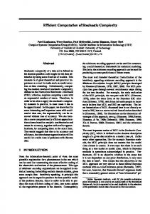
Fig. 1. Frequency and direction estimation using MUSIC with X and Xsp . Xsp has 258 nonzero elements. (L = 20 sensors, N = 30 samples, D = 3 signals with amplitudes a = [1 2 2], directions doa = [−20 10 40] and frequencies f = [−0.4 0.1 0.1], SNR=10, threshold th = 0.15)

MSE of FRE−Estimation using X and X

sp

−5

10

MSE

X

MSEXsp

−6

MSE

10

−7

10

−8

10

2

4

6

8

10

12 14 16 SNR MSE of DOA−Estimation using X and X

18

20

sp

0

10

MSEX MSEXsp

−1

10 MSE

Let Fm denote a DFT matrix of dimension m × m. Given a matrix A the operation (A) th describes the application of a threshold, i.e. all matrix elements of A, whose absolute values do not exceed a specific threshold th are set to zero (if |a ij | < th, then aij = 0; for all i, j). Applying the DFT (executed as FFT) to both sides of the data matrix X and applying a specific threshold results in a sparse matrix Xsp = (FN · X · FL )th . Using MUSIC/ESPRIT we estimate both frequencies and directions from this matrix Xsp , i.e. ES(Xsp ) resp. MU(Xsp ), and compare it to the estimation using the original data matrix X, i.e. ES(X) resp. MU(X). Of course, the number of non-zero elements increases, if the number of signals increases. Furthermore, the sparsity also depends on the chosen threshold and the SNR. Using Lanczos’ method to compute the SVD the sparsity of the matrix is directly related to the computational complexity. This is considered in section IV. Fig. 1 shows a first example. The simulation parameters are described in the caption of the figure. The sparsity of the resulting matrix Xsp is shown in the left part of the figure. The top right figure shows the results of the frequency estimation using MU(X) (dotted line) and MU(X sp ) (dashed line). The bottom right figure gives the results of the direction estimation using MU(X) (dotted line) and MU(X sp ) (dashed line). The results show that the accuracy of the estimates is roughly the same. In order to evaluate the accuracy of the estimates Fig. 2 shows the MSE (we show the mean of the D mean square errors) of the estimates for varying SNR using original data matrix X and sparse matrix X sp for 100 trials. Fig. 3 shows the mean value of the number of nonzero elements of the respective sparse matrices X sp obtained during these simulations. The threshold was chosen such that the number of nonzero elements is less than 200 (gradually decreasing the threshold for increasing SNR). We see that the estimation quality is retained for the sparse matrix.

20

0.2

−2

10

−3

10

2

4

6

8

10

12

14

16

18

20

SNR

Fig. 2. MSE of frequency and direction estimation with ESPRIT using original data matrix X and sparse matrix Xsp (L = 20, N = 30, a = [1 1 1], doa = [−20 10 40], f = [−0.4 0.1 0.3]) .

are constructed. The construction of these Hankel matrices using a column and a row of X, respectively, is illustrated in Fig. 4. For frequency estimation (see top of Fig. 4) an arbitrary column X(:, ), which has N elements, is separated into two parts. The first part contains the 1st to the N n -th element of X(:, ), i.e. c = X(1 : Nn , ), and the second part contains

Number of non−zero elements of X

sp

(of N*L=600 matrix elements)

sample is needed at each sensor to do the estimation, e.g. in wireless sensor networks, where the data samples need to be transmitted to a common processing unit accomplishing the estimations. A comparison between the accuracy of the estimation using matrix X and the estimation using Hankel matrices X f H and XdH is shown in Figure 5. The MSE of the frequency and the direction estimations with ESPRIT method using the Hankel matrices ES(Xf H ) and ES(XdH ), is compared to the MSE of the frequency and the direction estimations with ESPRIT method using the original data matrix ES(X).

600

non−zero elements

500

400

300

200

100

0

2

4

6

8

10

12

14

16

18

20

MSE of FRE−Estimation using X, XfH and XfHsp

−5

10

SNR

MSEX MSE

XfH

MSE

Fig. 3. Mean value of the number of nonzero elements in the matrices Xsp for the simulations done in Fig. 2.

MSE

XfHsp

−10

10

2

4

0

6 8 10 12 14 16 SNR MSE of DOA−Estimation using X, XdH and XdHsp

18

20

10

MSE

X

MSE

−2

MSE

10

XdH

MSEXdHsp −4

10

−6

10

2

4

6

8

10

12

14

16

18

20

SNR

Fig. 5. MSE of frequency estimation using Hankel matrix Xf H (MSEXf H ) and sparse matrix Xf Hsp (MSEXf Hsp ) and MSE of direction estimation using Hankel matrix XdH (MSEXdH ) and sparse matrix XdHsp (MSEXdHsp ) compared to MSE of frequency and direction estimation using data matrix X (MSEX ).(a = [1 1 1]; N = 64; L = 60; doa = [−20 10 40]; f = [−0.4 0.1 0.3]; Nn = 40; Ll = 40; z = 100).

non−zero elements

the Nn -th to the N -th element of X(:, ), i.e. r = X(N n : N, ), where Nn > (N − Nn + 1). The Nn × (N − Nn + 1) Hankel matrix Xf H has c as its first column and r as its last row. The Hankel matrix X dH for direction estimation can be constructed in the same way from a row X(g, :) and replacing N by L and Nn by L (see bottom of Fig. 4). Remark: The number of resolvable directions/frequencies is reduced to L − L  and N − Nn . Furthermore the number of sensors L and the number of samples N needs to be significantly higher than for the estimation using X in order to have sufficient data available. In case of frequency estimation this problem can be circumvented by just using more samples at a sensor. In case of direction estimation an increased number of sensors would be necessary, which is usually difficult to realize. On the other hand, it is advantageous that only one

Number of non−zero elements of XfHsp (of 3920 matrix elements)

3000 2000 1000 0

non−zero elements

Fig. 4. Constructing the Hankel matrices Xf H and XdH from the data matrix X. Application of DFTs and thresholding to these matrices is also shown.

2

4 6 8 10 12 14 16 18 SNR Number of non−zero elements of XdHsp (of 3280 matrix elements)

20

3000 2000 1000 0

2

4

6

8

10

12

14

16

18

20

SNR

Fig. 6. Mean value of the number of nonzero elements in the matrices Xf Hsp and XdHsp for the simulations done in Fig. 5.

Using the Hankel matrices X f H and XdH results in a reduced estimation accuracy compared to the estimation using

the matrix X. However, using the Hankel matrices X f H and XdH requires significantly less computations (see section IV). Analog to Sec. III-A, the DFT (FFT) is applied to both sides of the matrices Xf H and XdH (see right part of Fig. 4). Again, all elements not exceeding a threshold th are set to zero, which leads to the sparse matrices X f Hsp and XdHsp (note that the Hankel structure is lost for these matrices). At last the ES(Xf Hsp ) and ES(XdHsp ) will be used to estimate frequencies and directions. Fig. 5 shows the comparison of the MSE and Fig. 6 the number of nonzero elements. Here we used a constant threshold for the construction of the sparse matrices Xf Hsp and XdHsp (therefore, the number of nonzero elements decreases with increasing SNR). Now, the MSE is almost constant for increasing SNR. Therefore, a reduction of the computational complexity can be obtained for increasing SNR, if a certain estimation accuracy is sufficient. IV. C OMPUTATIONAL COMPLEXITY Complexity analysis of the used algorithms, like e.g. FFT and Lanczos bidiagonalization are given in this section. The bidiagonalization step is the dominant task in our algorithms. All following steps (Golub Kahan step [10], application of MUSIC/ESPRIT after the SVD) are common to all algorithms. Based on these assumptions we analyze how many operations can be saved with the presented approaches. A. FFT complexity Computing the 2D-DFT, i.e. F N · X · FL , by applying FFTs to the rows and the columns of matrix X needs: N L log2 N · L + log2 L · N (7) 2 2 multiplications. B. Complexity of Lanczos bidiagonalization The number of required multiplications for the Lanczos bidiagonalization depends on the structure of the matrix X [11]: Lanczos bidiagonalization of a dense matrix: For each iteration (N L+3N )+(N L+3L) multiplications are required. L iterations are performed, which sums up to [(N L + 3N ) + (N L + 3L)]L

(8)

multiplications. Lanczos bidiagonalization of sparse matrix: For each iteration (nZ + 3N ) + (nZ + 3L) multiplications are required. Because of the sparsity of the matrix, where the number of non-zero elements is n Z , only nZ multiplications are required for the matrix vector multiplication. Thus, there are totally [(nZ + 3N ) + (nZ + 3L)]L = 2nZ L + 3N L + 3L2

(9)

multiplications required. Lanczos bidiagonalization of Hankel matrix: A cyclic matrix Hc can be constructed from a N ×L Hankel matrix H. The

dimension of H c will be (N +L−1)×(N +L−1). y = Hx is ¯ , where ¯ = Hc x executed by the matrix vector multiplication y ¯ = [y y
]T and x ¯ = [x 0]T . Here, vector y has N elements, y vector y
has L − 1 elements, while vector x has L elements and vector 0 has N − 1 elements. Since Hc is cyclic, Hc = F−1 N +L−1 ΛFN +L−1 , where Λ is a diagonal matrix with diag(Λ) = F N +L−1 Hc (:, 1). Therefore ¯ = F−1 ¯ = F−1 ¯ = Hc x y N +L−1 ΛFN +L−1 x N +L−1 ΛxF = −1 FN +L−1 xFΛ . ¯ using FFT needs Computing xF = FN +L−1 x (N +L−1) log2 (N + L − 1) multiplications. Then x FΛ = ΛxF 2 ¯ = F−1 costs (N + L − 1) multiplications. At last y N +L−1 xFΛ (N +L−1) requires log (N + L − 1) multiplications. Therefore, 2 2 the complexity of the Hankel matrix vector multiplication is: (N + L − 1) log2 (N + L − 1) 2 + (N + L − 1) (N + L − 1) log2 (N + L − 1) + 2 = (N + L − 1)[1 + log2 (N + L − 1)]

nH =

(10)

For the Lanczos bidiagonalization with Hankel matrix, the N L multiplications in Eq. (8) can be replaced with n H operations of Eq. (10). Thus there are [(nH + 3N ) + (nH + 3L)]L = 2nH L + 3N L + 3L2

(11)

multiplications required. C. Comparison A comparison of the computational complexity of the different methods is given in Tab. 1 and Tab. 2. C1 is the computational complexity of the approach presented in Sec. III-A (using X and X sp ), while C2 is the computational complexity of the Hankel method presented in Sec. III-B (using Xf H/dH and Xf Hsp/dHsp ). Note, that in the case of C2 we have to execute the computations for both Hankel matrices. The column FFT shows the complexity of the 2D-DFT computed by FFTs. The column LanBi shows the complexity of the Lanczos bidiagonalization using the dense matrices. The column FFT/th/LanBi shows the complexity of the preprocessing step and the Lanczos bidiagonalization of the resulting sparse matrices. The column LanHankel shows the complexity of the Lanczos bidiagonalization exploiting the Hankel structure of the two Hankel matrices. Below the name of the procedure the tables also show the matrices to which the procedures are applied. We note that: 1) The computational complexities of FFT, LanBi, and LanHankel do not change if the threshold changes. No threshold is used for LanBi and LanHankel when they compute the SVD of the original matrices. FFT is used for rough estimation or as a preprocessing step.

C1/105 th=0.1 th=0.15 C2/105 th=0.1 th=0.15

FFT X 0.112 0.112 FFT Xf H XdH 0.057 0.057

LanBi X 1.402 1.402 LanBi Xf H XdH 0.576 0.576

FFT/th/LanBi X Xsp 0.854 0.501 FFT/th/LanBi Xf H Xf Hsp XdH XdHsp 0.205 0.182

— — —

LanHankel Xf H XdH 0.312 0.312

Table 1. Comparison of the complexity with L = 32 sensors, Ll = 20, N = 64 samples, Nn = 40, and D = 3 incoming signals

C1/105 th=0.1 th=0.2 C2/105 th=0.1 th=0.2

FFT X 0.112 0.112 FFT Xf H XdH 0.057 0.057

LanBi X 1.402 1.402 LanBi Xf H XdH 0.576 0.576

FFT/th/LanBi X Xsp 1.203 0.702 FFT/th/LanBi Xf H Xf Hsp XdH XdHsp 0.347 0.229

— — —

LanHankel Xf H XdH 0.312 0.312

Table 2. Comparison of the complexity with L = 32 sensors, Ll = 20, N = 64 samples, Nn = 40, and D = 10 incoming signals

2) C2=C2f+C2d. C2f is the computational complexity for frequency estimation with the Hankel matrix X f H , while C2d is the computational complexity for direction estimation with the Hankel matrix X dH . 3) The required operations for FFT/th/LanBi will decrease, if the threshold increases. Note, however, that if the threshold would be increased too much, the estimation results would get worse. 4) C2 is always lower than C1. However, the computed estimation results of C2 (using Hankel matrices) are not as good as for C1 (see Fig. 5). 5) If there are more incoming signals, the non-zero elements in the matrices will also increase and, therefore, the computational complexity increases, too (Comparing Tab. 2 to Tab. 1). 6) The operations for LanHankel can be less than for FFT/th/LanBi (see Tab. 2). But with the growth of the threshold, the computational complexity of the FFT/th/LanBi becomes less than that of LanHankel, because of the increasing number of zero elements in the sparse matrix. V. C ONCLUSION In this paper we have shown that it is worthwhile to use a two-sided FFT of the data matrix as a preprocessing step for computing frequency and DOA estimates. Together with a threshold,this preprocessing results in a sparse matrix which can be favorably used by the Lanczos method computing the SVD/EVD of the matrix in the ESPRIT/MUSIC method. This results in a significantly reduced computational complexity while the MSE of the estimates is almost retained. The frequencies and DOAs can also be obtained from the samples of one sensor and one sample of all sensors,

respectively, building Hankel matrices from these samples and then applying ESPRIT/MUSIC. This also results in an significant reduction of the computational complexity but yields significantly worse MSE. Applying the preprocessing (twosided FFT/threshold) to the Hankel matrices is also possible, but the computational complexity is only slightly reduced in specific cases, since the Hankel structure is destroyed by the preprocessing (it replaces Hankel structure by sparseness). In future work the choice of the threshold must be investigated more carefully, since it is directly related to the sparseness and the efficiency of the method. Furthermore, the use of a single snapshot or only one sensor is the extreme case. We can also take a subset of the sensors or a subset of the samples at each sensor and construct block Hankel matrices in order to increase the accuracy while still decreasing the number of required data samples/sensors and the computational complexity. R EFERENCES [1] S. Haykin: Cognitive Radio: Brain-Empowered Wireless Communications IEEE Journal on Selected Areas in Communications, Vol. 23, No.2, February 2005 [2] A. Veen, M. Vanderveen, A. Paulraj, L. Tao and H.K.Kwan: Joint Angle and Delay Estimation Using Shift-Invariance Techniques IEEE Transactions on Signal Processing, Vol. 46, No. 2, February 1998 [3] R.O. Schmidt: Multiple Emitter Location and Signal Parameter Estimation. IEEE Trans. Antennas Propagation, Vol. AP-34 (March 1986), pp.276-280. [4] R. Suleesathira: Close direction of arrival estimation for multiple narrowband sources Signal Processing and Its Applications, 2003. Proceedings. Seventh International Symposium on Volume 2, 1-4 July 2003 [5] R. Roy, A. Paulraj, T. Kailath: ESPRIT–A subspace rotation approach to estimation of parameters of cisoids in noise. IEEE Transactions on Acoustics, Speech and Signal Processing, Volume 34, Issue 5, Oct 1986 Page(s):1340 - 1342. [6] A. Lemma, A. Veen, and E. Deprettere: Analysis of Joint AngleFrequency Estimation Using ESPRIT IEEE Transactions on Signal Processing, Vol. 51, No. 5, May 2003 [7] L. Tao, H.K.Kwan: A Novel Approach To Fast DOA Estimation Of Multiple Spatial Narrowband Signals Department of Electronic Engineering and Information Science Anhui University; Department of Electrical and Computer Engineering University of Windsor [8] Y. He, K. Hueske, J. G¨otze, E. Coesmeier: Matrix-Vector Based FFT on SDR Architectures, Kleinheubacher Tagung, KH2007-C-004 [9] J. Goetze, A. Veen: On-Line Subspace Estimation Using a Schur-Type Method, IEEE Transactions on Signal Processing, Vol. 44, No. 6, June 1996 [10] G. Golub, C. Van Loan: Matrix Computations, Johns Hopkins Univ. Press, 3rd Edition, 1996 [11] P. Comon, G. H. Golub: Tracking a Few Extreme Singular Values and Vectors in Signal Processing, Proceedings of the IEEE, vol. 78, No. 8, August 1990 [12] G. Xu, Y. Cho and T. Kailath: Application of Fast Subspace Decomposition to Signal Processing and Communication Problems IEEE Transactions on Signal Processing, Vol. 42, No. 6, June 1994 [13] M. Zoltowski and C. Mathews: Real-Time Frequency and 2-D Angle Estimation with Sub-Nyquist Spatio-Temporal Sampling IEEE Transactions on Signal Processing, Vol. 42, No. 10, October 1994 [14] J. Lin, W. Fang, Y. Wang and J. Chen: FSF MUSIC for Joint DOA and Frequency Estimation and Its Performance Analysis IEEE Transactions on Signal Processing, Vol. 54, No. 12, December 2006 [15] P. Stoica, R. Moses: Spectral Analysis of Signals Prentice Hall (2005).