Efficient Computation of Trade-Off Skylines - Semantic Scholar

Efficient Computation of Trade-Off Skylines Christoph Lofi

Ulrich Güntzer

Wolf-Tilo Balke

Institute for Information Systems Mühlenpfordtstr. 23 38104 Braunschweig, Germany

Institute of Computer Science University of Tübingen 72076 Tübingen, Germany

Institute for Information Systems Mühlenpfordtstr. 23 38104 Braunschweig, Germany

[email protected]

ulrich.guentzer@informatik. uni-tuebingen.de

[email protected]

ABSTRACT When selecting alternatives from large amounts of data, trade-offs play a vital role in everyday decision making. In databases this is primarily reflected by the top-k retrieval paradigm. But recently it has been convincingly argued that it is almost impossible for users to provide meaningful scoring functions for top-k retrieval, subsequently leading to the adoption of the skyline paradigm. Here users just specify the relevant attributes in a query and all suboptimal alternatives are filtered following the Pareto semantics. Up to now the intuitive concept of compensation, however, cannot be used in skyline queries, which also contributes to the often unmanageably large result set sizes. In this paper we discuss an innovative and efficient method for computing skylines allowing the use of qualitative trade-offs. Such trade-offs compare examples from the database on a focused subset of attributes. Thus, users can provide information on how much they are willing to sacrifice to gain an improvement in some other attribute(s). Our contribution is the design of the first skyline algorithm allowing for qualitative compensation across attributes. Moreover, we also provide an novel trade-off representation structure to speed up retrieval. Indeed our experiments show efficient performance allowing for focused skyline sets in practical applications. Moreover, we show that the necessary amount of object comparisons can be sped up by an order of magnitude using our indexing techniques.

Categories and Subject Descriptors H.3.3 [Information Systems]: Information Search and Retrieval.

General Terms Algorithms, Human Factors

Keywords Skyline Queries, Preferences, Trade-off Management.

1. INTRODUCTION Recently skyline queries have successfully implemented the concept of Pareto optimality for filtering suboptimal database items. Any query result item can be safely ignored, if there exists some item that simply shows better values with respect to all query attributes: we say the ignored item is „dominated’. This is indeed a very intuitive concept. If for example two car dealers in the

Permission to make digital or hard copies of all or part of this work for personal or classroom use is granted without fee provided that copies are not made or distributed for profit or commercial advantage and that copies bear this notice and the full citation on the first page. To copy otherwise, to republish, to post on servers or to redistribute to lists, requires prior specific permission and/or a fee. EDBT 2010, March 22-26, 2010, Lausanne, Switzerland. Copyright 2010 ACM 978-1-60558-945-9/10/0003 ...$10.00.

neighborhood offer exactly the same model (with same warranties, etc.) at different prices, why should one want to consider the more expensive car? Furthermore, user preferences for skyline queries only have to be specified within each attribute (cheaper price, stronger engine, favorite color), which makes the paradigm intuitive to use. And while in most works on skyline queries only numerical domains and preferences are considered [3][11][15], skylining can even be extended to respect categorical preference (e.g. on colors) modeled as partial orders [12][4]. The focus on individual attribute domains and the complete fairness of the Pareto paradigm are major advantages of skyline queries. However, this also induces some shortcomings. Skylines completely lack the ability to relate attribute domains to each other and thus disallow compensation, weighting or ranking between domains. This often results in large amounts of incomparable objects and generally causes skylines results to be rather large, especially in the case of anti-correlated attributes. It has been shown that already for only 5 to 10 attributes, skylines can easily contain 30% or more of the entire database instance [2][3][7][8] and thus tend to be unmanageable. In order to decrease skyline sizes, there have recently been several approaches to rank skyline items according to some structural characteristics like counting how many other items does each skyline item dominate [4][5], or in how many subspace skylines each skyline item is present [17], etc. For the latter approaches, a large number of subspace skylines have to be computed, often employing „sky-cube‟-like algorithms [17][16]. However, it is not quite clear whether those structural properties are really related to the usefulness of items and will be helpful for the user. In contrast to merely structural approaches, a more user-centered focusing of the skyline set can be archived by incorporating feedback information provided by the user, thus introducing an additional layer of personalization. Most prominent among these approaches are techniques allowing users to interactively modify and extend their preferences in a cooperative fashion like [6] or [13]. In particular, users might consider some attributes to be more important than others. For example, [13] allows users to provide a total order for attributes; the evaluation then focuses on prioritized subspaces. The alternative approach to query personalization is Top-K Retrieval [10] paying particular attention to weightings of attributes. For each item high values in some attribute(s) may compensate for shortcomings with respect to other attributes following some scoring function (also called a utility function). Unfortunately, this compensation feature is not very intuitive to use. For instance, the semantics of an expression like “0.4*price + 0.8*color + 0.2* performance” is not intuitively understandable by most users. However, none of the mentioned approaches are able to support simple and natural trade-offs or compromises, which real world sales persons use every day. Consider, for example, three cars: let

item 𝐴 be a „blue metallic‟ car for $18000 and item 𝐵 be a „blue‟ car for $17000, accompanied by a preference favoring cheaper cars and metallic colors. Looking at the ranking on attribute level, both cars are incomparable with respect to the Pareto order: one car is cheaper, the other has the preferred color. In this scenario, a natural question of a car dealer would be, whether the customer is willing to compromise on those attributes, i.e. if he/she is willing to pay an additional $1000 for the metallic paint job (we call such compromises trade-offs). If the answer is yes, then item A is the better choice and would dominate item 𝐵 with respect to a tradeoff enhanced Pareto order. Still, if some item 𝐶 like a „blue‟ car for $15000 exists, 𝐴 and 𝐶 would remain incomparable as the premium for the metallic color on that car 𝐶 is larger than the said $1000 the user is willing to pay. From the viewpoint of order theory, the logical implications and problems of trade-off enhanced Pareto orders were already discussed in detail in our previous work [1]. Moreover, in [14] we presented a simple criterion for checking whether a set of trade-offs and attribute preferences are consistent and non-conflicting.

Our paper is structured as follows: we introduce basic theoretical concepts in section 2, starting with a formal definition of tradeoffs and corresponding trade-off skylines. We identify the object domination check as the crucial operation when adding trade-offs to the skyline paradigm. In section 3, we introduce our novel algorithm for efficiently computing the trade-off enhanced skyline. The main innovation is our data structure for computing the object domination check. The skyline algorithm and the corresponding representation structure is extensively evaluated in section 4. We show the effectiveness of the skyline reduction gained by trade-offs on real world data sets, and our algorithm‟s efficient run times suitable for real-life applications. We conclude our work in section 4.3 with a short summary and outlook.

However, actually computing a trade-off enhanced skyline efficiently from this order has still been impossible. This is because in contrast to Pareto orders, the trade-off enhanced order loses the characteristic of seperability [9] regarding the individual attributes. However, exactly this characteristic allows for building efficient skyline algorithms. In particular, when checking any two objects 𝐴 and 𝐵 for domination a skyline algorithms does not have to materialize the separable Pareto order. But any two items can be simply checked for domination componentwise: If attribute values of item A are better or equal regarding each attribute than item 𝐵‟s (with „strictly better‟ in at least one), then A dominates B and 𝐵 can be pruned from the skyline. Moreover, if two items only differ with respect to a single attribute the test for domination is even simpler due to the ceteris-paribus („all-else-being-equal‟) semantics, see e.g., [9].

Assume a database relation 𝑅 ⊆ 𝐷1 × … × 𝐷𝑛 on 𝑛 attributes.

In contrast to preferences, trade-offs always span over several attributes. For instance our example of a metallic paint job for $1000 tightly links the price attribute to the color. Now a componentwise comparison can still sort out all Pareto-dominated items, but as soon as the price of two items differs by at most $1000, a domination regarding the color attribute might be compensated for. This has to be checked individually (and thus inefficiently) for all trade-off pair. While for a single trade-off this test is still relatively inexpensive, introducing multiple trade-offs („Would you pay more for a stronger engine?‟) will inevitably lead to a complex order where attributes are intrinsically linked. But simply materializing the trade-off enhanced Pareto order is not possible for efficient domination checks. Therefore, until now no algorithm for computing skylines enhanced by trade-offs is known. In this paper we present the first skyline algorithm able to integrate the intuitive concept of trade-offs into database retrieval. Our algorithm always correctly computes the complete trade-off skyline and thus offers effective means for personalization. The contribution of this paper is that these characteristics can be obtained by materializing only a simple and non-redundant auxiliary trade-off representation structure. This contribution is twofold: on one hand, more information about the user can be consistently integrated into the retrieval process and thus be used to personalize the result set. On the other hand, the result sets are reduced without any arbitrary assumptions like „an item is better, if it dominates more other items‟[4][5] or „good items appear in more subspace skylines‟ [17].

2. BASIC CONCEPTS A complete order theoretical framework for preference structures is given in [1]. To be self-contained we will briefly reiterate the basic definitions and notation as they will be needed later.

2.1 Pareto Skylines 





A preference 𝑃𝑖 on an attribute 𝐴𝑖 with domain 𝐷𝑖 is a strict partial order over 𝐷𝑖 . If some attribute value 𝑎 ∈ 𝐷𝑖 is preferred over another value 𝑏 ∈ 𝐷𝑖 , then 𝑎, 𝑏 ∈ 𝑃𝑖 . This is written as 𝑎 >𝑖 𝑏 (reads as “𝑎 dominates 𝑏 wrt. to 𝑃𝑖 ”). Analogously, an equivalence 𝑄𝑖 is an equivalence relation on 𝐷𝑖 compatible with 𝑃𝑖 . If two attribute values 𝑎, 𝑏 ∈ 𝐷𝑖 are equivalent, i.e. 𝑎, 𝑏 ∈ 𝑄𝑖 , we write 𝑎 ≈𝑖 𝑏. Finally, if an attribute value 𝑎 ∈ 𝐷𝑖 is either preferred over or equivalent to another value 𝑏 ∈ 𝐷𝑖 , we write 𝑎 ≳𝑖 𝑏.

As an example, assume some transitive preferences for buying a car considering the attributes price, color, horsepower, and air conditioning as illustrated in Figure 1: $14000

Blue Metallic

With

110 hp

$16000

Blue

100 hp

$18000 $20000

White

Without

80 hp

Price

Color

A/C

Horsepower

Figure 1. Some preferences within the domain of cars To compute the skyline, the attribute preferences can be aggregated with respect to the Pareto semantics (so called Pareto aggregation) resulting in the full product order 𝑃. This order can then be used to test whether an object 𝑜1 from the database dominates any other object 𝑜2 (which is the case if 𝑜1 shows better or at least equal performance regarding all attributes than 𝑜2 ): Definition 1: full product order 𝑷 For 𝑃 ⊆ (𝐷1 × … × 𝐷𝑛 ) × (𝐷1 × … × 𝐷𝑛 ) and for any 𝑜1 , 𝑜2 ∈ (𝐷1 × … × 𝐷𝑛 ), 𝑜1 , 𝑜2 ∈ 𝑃 denoted by 𝑜1 >𝑃 𝑜2 is defined by ∀ 𝑖 ∈ 1, … , 𝑛 : o1,i ≳𝑖 o2,i ∧ ∃ 𝑖 ∈ {1, … 𝑛}: o1,i >𝑖 o2,i .  The skyline of 𝑅 is then defined as all non-dominated objects of the database 𝑅 with respect to the full product order:

Definition 2: Pareto skyline

Definition 3: trade-off skyline

𝑆𝑘𝑦 ≔ 𝑜2 ∈ 𝑅 ¬∃ 𝑜1 ∶ 𝑜1 >𝑃 𝑜2 }



(see e.g., [11]).

Note that product orders quickly grow very large with increasing number of attributes and domain cardinalities. However, for Pareto skyline computation it is not really necessary to materialize the full product order. For testing whether 𝑜1 >𝑃 𝑜2 holds, it is only necessary to compare the objects componentwise using the individual attribute preferences. The ability to perform the dominance check with respect to the product order by separately testing each component is called separability and is heavily exploited by all existing skyline algorithms, see e.g. [2][3][11][15].

2.2 Trade-Off Skylines



𝑆𝑘𝑦 ≔ 𝑜2 ∈ 𝑅 ¬∃ 𝑜1 ∶ 𝑜1 >T 𝑜2 }

This new criterion respects all trade-offs in 𝑇, but of course has to also respect all original Pareto preferences, too. Additionally, it has to also mind all interactions between trade-offs and Pareto preferences, which are given by the transitive closure of all preferences and trade-offs. However, this new order and the resulting check criterion are not separable anymore, i.e. the information provided by the trade-offs and their interactions cannot be mapped back to the attribute preferences without losing information (and thus, simple, attribute based comparisons are not sufficient anymore).

Trade-offs can be considered as a user decision between two sample objects focusing on a subset of the available attributes. For example, considering the domain of cars, a user could focus on the attributes color and price. A trade-off then describes in a qualitative fashion how much a user is willing to sacrifice in some dimension(s) to gain better performance in some other dimension(s) on the basis of a practical example. A possible trade-off 𝑡1 could be: “I would prefer a car for $18000 with a metallic blue paint job over a car for $16000 with a plain blue paint job.” We write 𝑡1 : = $18000, 𝑏𝑙𝑢𝑒 𝑚𝑒𝑡𝑎𝑙𝑙𝑖𝑐 ⊳ $16000, 𝑏𝑙𝑢𝑒 .

2.2.1 Trade-Off Dominance Relationships

More formally, a trade-off 𝑡 is always defined over a set of attributes given by respective indexes denoted as 𝜇 ⊆ 1, … , 𝑛 (see Figure 2 for the example trade-off 𝑡 defined over attributes 𝐴2 , 𝐴3 , and 𝐴4 ). To further simplify notation, let 𝐷𝜇 ∶= ⨉ 𝐷𝑖 and

In the following we will show inductively how to construct >𝐓 .

𝑖∈𝜇

𝜇 ≔ 1, … , 𝑛 ∖ 𝜇. Then, a trade-off is a relationship between two tuples 𝑥, 𝑦 ∈ 𝐷𝜇 denoted as 𝑡 ∶= (𝑥 ⊳ 𝑦). Obviously the two components of a trade-off 𝑥 and 𝑦 have to be in incomparable, i.e. no domination relationship 𝑥 ≥𝑃 𝑦, nor 𝑥 ≥𝑃 𝑦 exists between them. Each trade-off is defined on an individual attribute set 𝜇, i.e. some 𝑡1 may be defined on 𝜇1 and 𝑡2 on 𝜇2 .

⊳

A1 A2 A 3 A4 A5 y t1 x μ1 Figure 2. Trade-off t on 𝝁 ∶= {𝟐, 𝟑, 𝟒}

The strict pre-order >𝐓 is defined as the smallest preorder containing the full product order induced by the Pareto semantics, enhanced by all additional domination relationships induced by individual trade-offs or arbitrary combinations of trade-offs in 𝑻 (completed using the ceteris paribus semantics).  For a set 𝑇 ≔ {𝑡1 : = (𝑥1 ⊳ 𝑦2 )} containing only a single trade-off the construction is straightforward: given two objects 𝑜1 and 𝑜2 , 𝑜1 may either dominate 𝑜2 according to the original Pareto semantics or by actually applying the trade-off using both ceteris paribus and Pareto semantics. The trade-off can only be applied, if for all attributes the trade-off is defined on: 𝑜1 dominates the attribute values of the first trade-off component 𝑥1 and the attribute values of the second component 𝑦1 dominate 𝑜2 . Moreover, it is easy to see that a single trade-off can only be applied once [14]. Formally: Proposition 1: constructing 𝒐𝟏 >𝐓 𝒐𝟐 with 𝑻 = 𝟏 For any 𝑜1 , 𝑜2 ∈ 𝐷{1,…,𝑛} and a single trade-off 𝑥1 ⊳ 𝑦2 : 𝑜1 >T 𝑜2 holds, if ∀𝑖 ∈ 𝜇 ∶ 𝑜1,𝑖 ≳𝑖 𝑥1,𝑖 ∧ 𝑦1,𝑖 ≳𝑖 𝑜2,𝑖 𝑜1 >𝑃 𝑜2 ∨  ∧ ∀𝑖 ∈ 𝜇: 𝑜1,𝑖 ≳𝑖 𝑜2,𝑖 Figure 3 visualizes this concept (assuming 4-attribute objects and a 2-attribute trade-off with 𝜇 = {1, 2}). Please note that all comparisons needed are component-wise analogous to the case of Pareto skylines and thus are efficient to perform. μ o1 ≳

x1 ≳

≳

⊳

y1 ≳

≳

Assuming a set of trade-offs 𝑇, the resulting skyline analogously to Pareto skylines consists of all non-dominated objects of 𝑅 with respect to the new domination relationships induced by all the given trade-offs. It is denoted with > 𝑇 in the following (reads as “dominates with respect to the trade-offs in 𝑇”, see the following subsection for a formalization):

Definition 4: trade-off domination relationships

≳

Trade-offs usually induce new domination relationships between database items augmenting the full product order and thus also the final skyline. In particular, given the above sample trade-off all cars for $18000 with a blue metallic paint job (or even better features price- and color-wise) will dominate all cars for $16000 with a plain blue paint job (or even less preferred features) under the ceteris paribus semantics. For example, after introducing 𝑡1 , the car ($17000, 𝑏𝑙𝑢𝑒 𝑚𝑒𝑡𝑎𝑙𝑙𝑖𝑐, 100 ℎ𝑝, 𝑎/𝑐) would now dominate a (previously incomparable) car with the characteristics ($16000, 𝑤ℎ𝑖𝑡𝑒, 100 ℎ𝑝, 𝑛𝑜 𝑎/𝑐).

Analogously to >𝑃 , we can define > 𝑇 using the notion of domination relationships by providing an adequate comparison criterion.

o2 μ

Figure 3. 𝒐𝟏 >𝑻 𝒐𝟐 with a single trade-off For multiple trade-offs, >T is more difficult to construct. Let the set 𝑇 contain two trade-offs 𝑇: = {𝑡1 ≔ 𝑥1 ⊳ 𝑦1 , 𝑡2 ≔ (𝑥2 ⊳ 𝑦2 )}. Now, 𝑜1 dominates 𝑜2 in either of the following cases:

≳

y1

x2 ⊳

y2

Refer to Figure 4 for an illustration of the trade-off sequence 𝑡1 ∘ 𝑡2 . Thus, to fully capture the semantics of 𝑜1 >T 𝑜2 for two tradeoffs, all four previously mentioned cases need to be considered, i.e. testing for Pareto dominance of 𝑜1 and 𝑜2 , dominance by considering any single one trade-off, and finally considering all sequences possible with both two trade-offs. Obviously, the complexity for expressing 𝑜1 >T 𝑜2 thus can exponentially increase with the number of trade-offs. For 𝑚 tradeoffs, 𝑜1 > 𝑇 𝑜2 holds in any of the following cases     

If 𝑜1 dominates 𝑜2 by plain Pareto semantics If 𝑜1 dominates 𝑜2 by any single trade-off If 𝑜1 dominates 𝑜2 by any possible trade-off sequence which can be formed using two trade-offs … If 𝑜1 dominates 𝑜2 by any possible trade-off sequence which can be formed using m trade-offs

≳

o2

μ1 ∩ μ2

μ1 ∪ μ2

Figure 4. 𝒐𝟏 >𝑻 𝒐𝟐 with two trade-offs 𝒕𝟏 ∘ 𝒕𝟐

2.2.2 Merging Trade-Off Tuples For building an efficient algorithm and ease notation for the theorem and proof in 2.2.3, we now introduce the concept of merging tuples (denoted by ↶). The idea is to merge two tuples with differing 𝜇-attribute sets and subsequently work on the resulting tradeoff. The merging operation is not commutative as a „dominant‟ tuple is merged with values of a „weaker‟ tuple. The merged tuple will have all attribute values where the dominant tuple is defined and all those attributes not defined by the dominant tuple will be completed with the weaker tuple‟s values. See Figure 5 for illustration.

μz z

∧ ∀𝑖 ∈ 𝜇1 ∪ 𝜇2 : 𝑜1,𝑖 ≳𝑖 𝑜2,𝑖 Of course as stated above, also all other possible sequences of trade-offs can be used to establish a domination relationship between 𝑜1 and 𝑜2 .

μ2 \μ1

≳

μ1 \μ2

≳

∈ 𝜇1 ∩ 𝜇2 : 𝑦1,𝑖 ≳𝑖 𝑥2,𝑖 ∈ 𝜇2 ∖ 𝜇1 : 𝑜1,𝑖 ≳𝑖 𝑥2,𝑖 ∈ 𝜇2 : 𝑦2,𝑖 ≳𝑖 𝑜2,𝑖 ∈ 𝜇1 ∖ 𝜇2 : 𝑦1,𝑖 ≳𝑖 𝑜2,𝑖

≳

∧ ∀𝑖 ∧ ∀𝑖 ∧ ∀𝑖 ∧ ∀𝑖

⊳

∀𝑖 ∈ 𝜇1 : 𝑜1,𝑖 ≳𝑖 𝑥1,𝑖

x1

≳

Given 𝑡1 = 𝑥1 ⊳ 𝑦1 with 𝜇1 and 𝑡2 = 𝑥2 ⊳ 𝑦2 with 𝜇2 . To show how the domination relationships are constructed, we will exemplify the forth case from above; the remaining cases are constructed analogously. Assume 𝑡1 and 𝑡2 can be applied in sequence 𝑡1 ∘ 𝑡2 , i.e. ∀𝑖 ∈ 𝜇1 ∩ 𝜇2 : 𝑦1,𝑖 ≳𝑖 𝑥2,𝑖 . Then, for any 𝑜1 , 𝑜2 ∈ 𝐷 1,…,𝑛 a domination relationship 𝑜1 >T 𝑜2 via a sequence 𝑡1 ∘ 𝑡2 holds, if

o1 ≳

Proposition 2: constructing 𝒐𝟏 >𝐓 𝒐𝟐 with 𝑻 = 𝟐:

μ2

μ1

≳

By applying simple Pareto semantics, i.e. 𝑜1 >𝑃 𝑜2 By applying trade-off 𝑡1 using ceteris paribus semantics, i.e. for attributes in 𝜇1 : 𝑜1 ≳𝑃 𝑥1 ∧ 𝑦1 ≳𝑃 𝑜2 and for all other attributes 𝑜1 ≳𝑃 𝑜2 (cf. proposition 1) 3. By applying trade-off 𝑡2 using ceteris paribus semantics, i.e. for attributes in 𝜇2 : 𝑜1 ≳𝑃 𝑥2 ∧ 𝑦2 ≳𝑃 𝑜2 and for all other attributes 𝑜1 ≳𝑃 𝑜2 (cf. proposition 1) 4. By applying both trade-offs 𝑡1 and 𝑡2 . In this case, both trade-offs need to be applied consecutively in order to establish a domination relationship between 𝑜1 and 𝑜2 , i.e. they form a trade-off sequence (consecutive tradeoff application will be denoted with ∘ in the following). In this case, several options may be possible: 𝑡1 ∘ 𝑡2 , and 𝑡2 ∘ 𝑡1 , but also 𝑡1 ∘ 𝑡2 ∘ 𝑡1 and (𝑡2 ∘ 𝑡1 ) ∘ 𝑡1 (Please note that no longer sequences exist for two consistent trade-offs, see [14] for more details). In general, a trade-off sequence 𝑡1 ∘ 𝑡2 is possible, if for all attributes appearing in both trade-offs, the second tuple of the first trade-off 𝑦1 component-wise dominates or equals the first tuple of the second trade-off 𝑥2 with respect to the attribute preferences, i.e. ∀𝑖 ∈ (𝜇1 ∩ 𝜇2 ) ∶ 𝑦1,𝑖 ≳𝑖 𝑥2,𝑖 . Formally, the concept of domination via trade-off sequences can be expressed as follows: 1. 2.

x μx x

z | ( μz \ μx)

Figure 5. Merged Tuple (𝒙 ↶ 𝒛) Definition 4: The Merge Operator ↶ : Let 𝜇x , 𝜇z ⊆ {1, … , 𝑛}. For 𝑥 ∈ 𝐷𝜇 𝑥 and 𝑧 ∈ 𝐷𝜇 𝑧 , the tuple 𝑥 ↶ 𝑧 is defined component-wise as: 𝑥 : 𝑖 ∈ 𝜇x (𝑥 ↶ 𝑧) ≔ 𝑢 𝑤𝑖𝑡ℎ 𝑢𝑖 = 𝑖  𝑧𝑖 : 𝑖 ∈ (𝜇z ∖ 𝜇𝑥 ) The merge operator is particularly helpful for simplifying the attribute-based notation of object domination criterions, because it allows performing the case-differentiation implicitly appearing in the criterions (when two or more trade-offs are involved). Using the new merge notation, now the condition for object domination via one single trade-off (Proposition 1) may be simplified by merging the non-affected parts of the objects under scrutiny directly into the trade-off conditions (and the separate consideration of attributes in 𝜇 and 𝜇 is not necessary anymore):

Proposition 1 (cont.): constructing 𝒐𝟏 >𝐓 𝒐𝟐 with the merge operator for 𝑻 = 𝟏 𝑜1 >T 𝑜2 ⇔ 𝑜1 >𝑃 𝑜2 ∨ 𝑜1 ≳𝑃 𝑥1 ↶ 𝑜1 ∧ 𝑦1 ↶ o1 ≳𝑃 𝑜2



An example using our trade-off 𝑡1 introduced above: 𝑡1 = $18000, 𝑏𝑙𝑢𝑒 𝑚𝑒𝑡𝑎𝑙𝑙𝑖𝑐 ⊳ $16000, 𝑏𝑙𝑢𝑒 is given in Figure 6. Assume that 𝑜1 dominates 𝑥1 with respect to all attributes in 𝜇1 . The trade-off components can now be merged on attributes in 𝜇1 with the values of 𝑜1 . Now the (artificially) created intermediate objects containing the trade-off values are in a proper domination relationship (𝑥1 ↶ 𝑜1 >T 𝑦1 ↶ o1 ) according to the tradeoff plus the ceteris paribus semantics (i.e. values in the nonaffected parts are equal). If now 𝑜2 is dominated by 𝑦1 ↶ o1 , it is also dominated by 𝑜1 via the trade-off 𝑡1 . Note, that only simple and separable domination checks -as already used in traditional skyline algorithms- are needed.

x1 ↶o1

$18000 blue metallic ⊳

⊳

=

=

y1 ↶o1

$16000

blue

a/c

80 hp

≳

≳

≳

≳

$16000

white

80 hp =

a/c

80 hp

2)

𝑜1 ≳𝑃 𝑥1 ↶ 𝑜1 ≡ ∀𝑖 ∈ 𝜇1 : 𝑜1,𝑖 ≳𝑖 𝑥1,𝑖 ∧ ∀𝑖 ∈ 𝜇1 : 𝑜1,𝑖 ≳𝑖 𝑜1,𝑖 ≡ ∀𝑖 ∈ 𝜇1 : 𝑜1,𝑖 ≳𝑖 𝑥1,𝑖 𝑦1 ↶ o1 ≳𝑃 𝑥2 ↶ 𝑦1 ↶ 𝑜1 ∀𝑖 ∈ 𝜇1 ∖ 𝜇2 : 𝑦1,𝑖 ≳𝑖 𝑦1,𝑖 ≡

≡ 3)

∧ ∀𝑖 ∈ 𝜇1 ∩ 𝜇2 : 𝑦1,𝑖 ≳𝑖 𝑥2,𝑖 ∧ ∀𝑖 ∈ 𝜇2 ∖ 𝜇1 : 𝑜1,𝑖 ≳𝑖 𝑥2,𝑖 ∧ ∀𝑖 ∈ 𝜇1 ∪ 𝜇2 : 𝑜1,𝑖 ≳𝑖 𝑜1,𝑖 ∀𝑖 ∈ 𝜇1 ∩ 𝜇2 : 𝑦1,𝑖 ≳𝑖 𝑥2,𝑖

∧ ∀𝑖 ∈ 𝜇2 ∖ 𝜇1 : 𝑜1,𝑖 ≳𝑖 𝑥2,𝑖 (𝑦2 ↶ 𝑦1 ↶ 𝑜1 ≳𝑃 𝑜2 ) ∀𝑖 ∈ 𝜇1 ∖ 𝜇2 : 𝑦1,𝑖 ≳𝑖 𝑜2,𝑖 ≡

∧ ∀𝑖 ∈ 𝜇2 : 𝑦2,𝑖 ≳𝑖 𝑜2,𝑖

μ2

μ1

no a/c 80 hp

x1 ↶o1

$18000 blue metallic

⊳

=

=

y1 ↶o1

$16000

blue

a/c

80 hp

=

≳

≳

=

x2 ↶ y1 ↶o1

$16000

blue

a/c

80 hp

=

⊳

⊳

=

y2 ↶ y1 ↶o1

$16000 blue metallic no a/c 80 hp

o2

$16000 blue metallic no a/c 80 hp

Transform each of the three clauses using the merge operator ↶ given in Proposition 2 (cont.) into component-wise comparisons

80 hp

≳

Proof for Proposition 2 (cont.): the component-wise dominance check is equivalent to a dominance check using merging

=

Of course we still have to show that the merging does not in any form alter our dominance checks as originally defined. For brevity we give the proof only for the more complex Proposition 2:

a/c

≳

These trade-offs can be applied in sequence as either as 𝑡1 ∘ 𝑡2 or 𝑡2 ∘ 𝑡1 . The common attribute is 𝑐𝑜𝑙𝑜𝑟, and in case of 𝑡1 ∘ 𝑡2 the value 𝑏𝑙𝑢𝑒 𝑚𝑒𝑡𝑎𝑙𝑙𝑖𝑐 allows for establishing the sequence. After applying both trade-offs in sequence, as illustrated in Figure 7 the car ($18000, 𝑏𝑙𝑢𝑒 𝑚𝑒𝑡𝑎𝑙𝑙𝑖𝑐, 80 ℎ𝑝, 𝑎/𝑐) dominates the second car ($16000, 𝑏𝑙𝑢𝑒 𝑚𝑒𝑡𝑎𝑙𝑙𝑖𝑐, 80 ℎ𝑝, 𝑛𝑜 𝑎/𝑐) via 𝑡1 ∘ 𝑡2 .

80 hp

=

$18000, 𝑏𝑙𝑢𝑒 𝑚𝑒𝑡𝑎𝑙𝑙𝑖𝑐 ⊳ $16000, 𝑏𝑙𝑢𝑒 𝑏𝑙𝑢𝑒, 𝑎/𝑐 ⊳ 𝑏𝑙𝑢𝑒 𝑚𝑒𝑡𝑎𝑙𝑙𝑖𝑐, 𝑛𝑜 𝑎/𝑐

≳



To also understanding this concept, consider again our example for two trade-offs 𝑡1 and 𝑡2 as follows:

≳

Proposition 2 (cont.): constructing 𝒐𝟏 >𝐓 𝒐𝟐 with the mergeoperator for 𝑻 = 𝟐

≳

$18000 blue metallic

⊳

Of course also the previous condition for 𝑡1 ∘ 𝑡2 in Proposition 2 may be rewritten using tuple merging. Here we can see the benefit of the merge operator: the need for case differentiation on different subsets combination of 𝜇1 and 𝜇2 is completely removed.

a/c

o1

μ1

𝑜1 >T 𝑜2 ⇐ 𝑜1 ≳𝑃 𝑥1 ↶ 𝑜1 ∧ 𝑦1 ↶ o1 ≳𝑃 𝑥2 ↶ 𝑦1 ↶ 𝑜1 ∧ (𝑦2 ↶ 𝑦1 ↶ 𝑜1 ≳𝑃 𝑜2 )

■

∧ ∀𝑖 ∈ 𝜇1 ∪ 𝜇2 : 𝑜1,𝑖 ≳𝑖 𝑜2,𝑖

Figure 6: 𝒐𝟏 >𝐓 𝒐𝟐 with trade-off $𝟏𝟖𝟎𝟎𝟎, 𝒃𝒍𝒖𝒆 𝒎𝒆𝒕𝒂𝒍𝒍𝒊𝒄 ⊳ $𝟏𝟔𝟎𝟎𝟎, 𝒃𝒍𝒖𝒆

𝑡1 = 𝑡2 =

1)

≳

μ1

a/c =

o2

≳

$18000 blue metallic ≳

o1

in order to create the comparison terms used in the original Proposition 2. All light-gray printed terms are trivially true and can be ignored. The six resulting component-based comparisons terms are exactly those given by the original Proposition 2.

Figure 7. 𝒐𝟏 >𝑻 𝒐𝟐 with two trade-offs 𝒕𝟏 ∘ 𝒕𝟐

2.2.3 Integrating Trade-Off Chains into Single Trade-offs When examining the previous example more closely, it can be observed that the comparisons between components of 𝑡1 and 𝑡2 are independent of 𝑜1 and 𝑜2 , i.e. the fact whether two trade-offs can be applied in sequence or not and which effects they have on object comparisons can be pre-computed independently of the database content. More generally, any valid trade-off sequence can be understood and handled as a single trade-off by checking for applicability and then combining the respective components. For example, trade-off sequence 𝑡1 ∘ 𝑡2 acts like a single trade-off 𝑡1∘2 ≔ (($18000, 𝑏𝑙𝑢𝑒 𝑚𝑒𝑡𝑎𝑙𝑙𝑖𝑐, 𝑎/𝑐) ⊳ ($16000, 𝑏𝑙𝑢𝑒 𝑚𝑒𝑡𝑎𝑙𝑙𝑖𝑐, 𝑛𝑜 𝑎/𝑐)), i.e. instead of testing 𝑜1 > 𝑇 𝑜2 with respect to the sequence 𝑡1 ∘ 𝑡2 , also 𝑜1 > 𝑇 𝑜2 with respect to the integrated trade-off 𝑡1∘2 could be tested. This new trade-off 𝑡1∘2 is defined as following:

Definition 5: trade-off integration

Algorithm 1: Basic Trade-Off Skyline Computation:

Assume that 𝑡1 ≔ (𝑥1 ⊳ y1 ) on 𝜇1 , and 𝑡2 ≔ (𝑥2 ⊳ y2 ) on 𝜇2 , and 𝑡1 and 𝑡2 can be applied in sequence, i.e. . ∀𝑖 ∈ 𝜇1 ∩ 𝜇2 : 𝑦1,𝑖 ≳𝑖 𝑥2,𝑖 . Then a new trade-off 𝑡1∘2 can be defined which is equivalent with respect to object domination to the tradeoff sequence 𝑡1 ∘ 𝑡2 . This integrated trade-off is given by:

Parameters:

If ∀𝑖 ∈ 𝜇1 ∩ 𝜇2 holds 𝑦1,𝑖 ≳𝑖 𝑥2,𝑖 then 𝑡1∘2 ≔ ( 𝑥1 ↶ 𝑥2 ⊳ y2 ↶ 𝑦1 )



Theorem 1: Integrating trade-off sequences into a single trade-off does not affect subsequent skyline computation. Proof (sketch): First consider the integration of two trade-offs: assume 𝑡1∘2 as a single trade-off 𝑡3 and use the domination criterion for a single trade-off as given by Proposition 1. This can be transformed to be equivalent to the component-wise domination criterion for two trade-offs as given by Proposition 2: 𝑜1 >T 𝑜2 with respect to 𝑡3 ≔ 𝑡1∘2 is given by Proposition 1 (cont.) as: 𝑜1 >T 𝑜2 ≡ 𝑜1 ≳𝑃 𝑥3 ↶ 𝑜1 ∧ 𝑦3 ↶ o1 ≳𝑃 𝑜2 Replace 𝑥3 and 𝑦3 with their definition as given by Definition 5 ≡ 𝑜1 ≳𝑃 (𝑥1 ↶ 𝑥2 ) ↶ 𝑜1 ∧ (y2 ↶ 𝑦1 ) ↶ o1 ≳𝑃 𝑜2 Transform both clauses to component-wise comparisons: ∀𝑖 ∈ 𝜇1 : 𝑜1,𝑖 ≳𝑖 𝑥1,𝑖 𝑜1 ≳𝑃 (𝑥1 ↶ 𝑥2 ) ↶ 𝑜1 ≡

∧ ∀𝑖 ∈ 𝜇2 ∖ 𝜇1 : 𝑜1,𝑖 ≳𝑖 𝑥2,𝑖 ∧ ∀𝑖 ∈ 𝜇1 : 𝑜1,𝑖 ≳𝑖 𝑜1,𝑖 ∀𝑖 ∈ 𝜇1 ∖ 𝜇2 : 𝑦1,𝑖 ≳𝑖 𝑜2,𝑖

(y2 ↶ 𝑦1 ) ↶ o1 ≳𝑃 𝑜2 ≡

∧ ∀𝑖 ∈ 𝜇2 : 𝑦2,𝑖 ≳𝑖 𝑜2,𝑖 ∧ ∀𝑖 ∈ 𝜇1 ∪ 𝜇2 : 𝑜1,𝑖 ≳𝑖 𝑜2,𝑖

Additionally, ∀𝑖 ∈ 𝜇1 ∩ 𝜇2 : 𝑦1,𝑖 ≳𝑖 𝑥2,𝑖 holds, since we assumed the existence of the trade-off chain to form 𝑡1∘2 . Thus, all six terms (and no additional ones) of the original Proposition 2 have been derived. The theorem then follows by induction over the numbers of trade-offs in the sequence. ■

3. THE TRADE-OFF SKYLINE In this section, we present the baseline algorithm for computing a trade-off skyline and introduce a basic tree-shaped representation structure for materializing trade-off chains.

3.1 A Basic Trade-Off Skyline Algorithm Obviously a trade-off skyline is a subset of the original Pareto skyline (as the definition of 𝑜1 > 𝑇 𝑜2 includes 𝑜1 >𝑃 𝑜2 ). Thus, a basic algorithm may first compute the Pareto skyline (by any one of the many popular algorithms) and then filter all additional objects which are dominated by another object via any trade-off sequence. Please note that this second domination check is much more expensive than the simple check for Pareto domination, thus interleaving Pareto and trade-off dominance checks generally leads to inferior performance. Checking the domination between objects with respect to trade-off sequences can be summarized as:  

Generate all integrated trade-offs representing all possible trade-off sequences 𝑜1 > 𝑇 𝑜2 holds, if applying any of the integrated tradeoffs leads to an domination relationship

When using the nested loop approach (as introduced by [11]), this results in the following basic algorithm:

  

Database relation 𝑅 on 𝑛 attributes 𝐴1 , … , 𝐴𝑛 Attribute preferences 𝑃1 , … , 𝑃n Set of trade-offs 𝑇

Algorithm: 1. Compute Pareto skyline 𝑠𝑘𝑦 with given database 𝑅 and preferences 𝑃1 , … , 𝑃n 2. Generate the set off all possible integrated trade-offs 𝑇′ 3. For all 𝑜1 ∈ 𝑠𝑘𝑦: 3.1. For all 𝑜2 ∈ 𝑠𝑘𝑦 ∧ 𝑜2 ≠ 𝑜1 : 3.1.1. If 𝑜1 > 𝑇 𝑜2 (tested using Algorithm 2) 3.1.1.1. Remove 𝑜2 from 𝑠𝑘𝑦 Algorithm 2: Basic Object Domination Test >𝑻 Parameters:  

Database objects 𝑜1 and 𝑜2 All possible integrated trade-offs 𝑇′

Returns: 𝑡𝑟𝑢𝑒 if 𝑜1 > 𝑇 𝑜2 , 𝑓𝑎𝑙𝑠𝑒 otherwise Algorithm: 1. For all trade-offs 𝑡𝑖 ≔ (𝑥 ⊳ 𝑦) ∈ 𝑇′ 1.1. If 𝑜1 ≳𝑃 𝑥 ↶ 𝑜1 ∧ 𝑦 ↶ o1 ≳𝑃 𝑜2 return 𝑡𝑟𝑢𝑒 (i.e.: 𝑜1 dominates 𝑜2 via 𝑡𝑖 , see Proposition 1 (cont.)) 2. Return 𝑓𝑎𝑙𝑠𝑒 The requirement for the set 𝑇′ is that each integrated trade-off (representing some trade-off sequence) for a given set of basic trade-offs 𝑇 is contained. While those sequences may only consist of |𝑇| different trade-offs, they may have arbitrary length (i.e. the same trade-off may appear even multiple times in a sequence) as long as each directly adjacent trade-off pair 𝑡𝑗 and 𝑡𝑗 +1 in that sequence fulfills the sequencing condition ∀𝑖 ∈ (𝜇j ∩ 𝜇j+1 ) ∶ 𝑦j,𝑖 ≳𝑖 𝑥j+1,𝑖 . Please note that sequences of unlimited length can only occur for inconsistent trade-off sets which can be efficiently tested and excluded before skyline computation (see [14] for theoretical results on possible sequence patterns, sequence finiteness, and the consistency test), thus the length of each tradeoff sequence and the number of sequences are both finite. Obviously, simply generating and testing all these integrated trade-offs without further optimizations is not very efficient. Thus, in the following we introduce a compact representation for performing these tests with the minimal possible efforts.

3.2 Representing Trade-Off Sequences The idea is to incrementally create a tree structure (called trading tree (𝑇𝑇𝑟𝑒𝑒) in the following) enumerating all currently possible trade-off sequences (represented by integrated trade-offs). In its basic version, the tree structure does not provide significant advantages over a simple list of all integrated trade-offs. However, the tree structure will enable our optimizations in section 3.3. Each node of the tree denotes a trade-off, which is either a user provided trade-off or some integrated trade-off representing a trade-off sequence (as described in Definition 5). Initially, the tree starts with a single, empty root trade-off 𝑡∅ : = ( ⊳ ) with empty 𝜇∅ : = ∅, i.e. nothing is traded. Then, trade-offs are inserted one by one from the set of all user trade-offs 𝑇. To complete the

tree, for each existing node we test whether the trade-off sequence it represents can be extended with the newly inserted user tradeoff (the root can always be extended, i.e. 𝑡∅ ∘ 𝑡𝑖 = 𝑡𝑖 ). Also, every newly created node needs to be extended with all previously inserted trade-offs if possible: Algorithm 3: Basic Algorithm for Trading Tree creation:

Now, consider a third trade-off: 𝑡3 ≔

$15000, 100 𝐻𝑃 ⊳ $14000, 80 𝐻𝑃 .

This trade-off can, for example, be applied in sequence with 𝑡2 , allowing the sequence 𝑡2 ∘ 𝑡3 . It cannot, however, be integrated with 𝑡1 (thus neither 𝑡1 ∘ 𝑡3 nor 𝑡2 ∘ 𝑡1 ∘ 𝑡3 is possible). Considering all possibilities, this results in the following tree (Figure 10):

Parameters: t1

t1∘2

Returns: A tree containing all integrated trade-offs possible with trade-off set 𝑇 and attribute preferences 𝑃1 , … , 𝑃n

t2

t2∘1

Algorithm:

t3

 

Attribute preferences 𝑃1 , … , 𝑃n Set of trade-offs 𝑇

t∅

1. 𝑇𝑇𝑟𝑒𝑒: = {𝑡∅ } 2. 𝑖𝑛𝑐𝑙𝑢𝑑𝑒𝑑𝑇: = ∅ 3. For each user trade-off 𝑡𝑖 ≔ (𝑥1 ⊳ 𝑦1 ) ∈ 𝑇 3.1. 𝑖𝑛𝑐𝑙𝑢𝑑𝑒𝑑𝑇 ≔ 𝑖𝑛𝑐𝑙𝑢𝑑𝑒𝑑𝑇 ∪ 𝑡𝑖 ; 𝑛𝑒𝑤𝑛𝑜𝑑𝑒𝑠 = ∅; 3.2. For each existing tree node 𝑡𝑜 ∈ 𝑇𝑇𝑟𝑒𝑒 3.2.1. Test whether 𝑡𝑜 ∘ 𝑡𝑖 is possible, i.e.: ∀𝑖 ∈ (𝜇1 ∩ 𝜇2 ) ∶ 𝑦1,𝑖 ≳𝑖 𝑥2,𝑖 3.2.1.1. Create integrated trade-off 𝑡𝑜∘𝑖 and add to 𝑇𝑇𝑟𝑒𝑒 by attaching to 𝑡𝑜 3.2.1.2. Add 𝑡𝑜∘𝑖 to 𝑛𝑒𝑤𝑛𝑜𝑑𝑒𝑠 3.3. For each newly created node 𝑡𝑛 ∈ 𝑛𝑒𝑤𝑛𝑜𝑑𝑒𝑠 3.3.1. For each user trade-off 𝑡𝑢 ∈ 𝑖𝑛𝑐𝑙𝑢𝑑𝑒𝑑𝑇 3.3.1.1. If 𝑡𝑛 ∘ 𝑡𝑢 is possible, i.e.: ∀𝑖 ∈ (𝜇n ∩ 𝜇u ) ∶ 𝑦n,𝑖 ≳𝑖 𝑥u,𝑖 3.3.1.1.1. Create integrated trade-off 𝑡𝑛∘𝑢 and add to 𝑇𝑇𝑟𝑒𝑒 by attaching to 𝑡𝑛 3.3.1.1.2. Add 𝑡𝑛∘𝑢 to 𝑛𝑒𝑤𝑛𝑜𝑑𝑒𝑠 As an example, consider the trade-offs 𝑡1 and 𝑡2 on {price, color} and {color, air conditioning} from above: 𝑡1 = 𝑡2 =

$18000, 𝑏𝑙𝑢𝑒 𝑚𝑒𝑡𝑎𝑙𝑙𝑖𝑐 ⊳ $16000, 𝑏𝑙𝑢𝑒 𝑏𝑙𝑢𝑒, 𝑎/𝑐 ⊳ 𝑏𝑙𝑢𝑒 𝑚𝑒𝑡𝑎𝑙𝑙𝑖𝑐, 𝑛𝑜 𝑎/𝑐

Let us insert 𝑡1 first and directly attach it to the root (see Figure 8). The integrated trade-off 𝑡1∘1 is obviously not possible (but would directly result in a cyclic inconsistency).

t∅

Figure 8. Basic TTree for 𝑻: = {𝒕𝟏 } Next, 𝑡2 is inserted and also attached to the root. Now, the node 𝑡1 has to be tested whether it can be extended, i.e. if a trade-off sequence 𝑡1 ∘ 𝑡2 is possible (c.f. Proposition 2). In our case, it is possible and thus the node 𝑡1∘2 is created as an integrated tradeoff (see Definition 5). Since the node 𝑡1∘2 is new, we still have to test whether this sequence can be extended to either form 𝑡1 ∘ 𝑡2 ∘ 𝑡1 or 𝑡1 ∘ 𝑡2 ∘ 𝑡2 , but evaluating the conditions only the first case is possible. The same procedure is also applied to the newly appended leaf node 𝑡2 . The resulting TTree is shown in figure 9. t1∘2

t2

t2∘1

t2∘3 t 3∘1

t 3∘1∘2

t 3∘1∘2 ∘1

t3∘2

Figure 10. Basic TTree for 𝑻 = {𝒕𝟏 , 𝒕𝟐 , 𝒕𝟑 } It can also be observed that each node within a branch represents an integrated trade-off sequence extending the sequences of all its ancestors. Still, each integrated trade-off has two distinct components: an upper part (called 𝑦 in Figure 2) and a lower part (called 𝑥 in Figure 2). When comparing the individual components of a node to the components of any of its ancestors, it can be observed that the complete values of any ancestor‟s upper part are by construction also contained in the upper part component of all its descendents (this directly follows from the definition of integrated trade-offs (Definition 5) and the merge-operation (Definition 4)). Thus, for each trade-off integrated into some existing trade-off, the ancestor‟s upper part component is only extended by values for previously undefined attributes. As soon as all attributes have been defined, the upper part component of all trade-offs in a branch becomes stable; integrating additional trade-offs into it, has no effects anymore. Thus, it is possible to store just the lower part component of trade-offs in the 𝑇𝑇𝑟𝑒𝑒 in order to save memory, and just link the first component from the respective parent. To integrate the trading tree into the basic skyline algorithm, Algorithm 3 has to be used in Algorithm 1 for computing all trade-off sequences, and the nodes of the tree are treated as the set of possible trade-offs.

3.3 Removing Redundancy from the Tree

t1

t1

t1∘2∘1

t1∘2 ∘1

t∅

Figure 9. Basic TTree for 𝑻: = {𝒕𝟏 , 𝒕𝟐 }

Although the previously described 𝑇𝑇𝑟𝑒𝑒 allows for systematically generating all possible trade-off relationships, it still tends to grow rather large. But taking a closer look, it still contains a lot of redundant information severely hampering the performance of domination check operations. In the following, we exploit some structural properties of the 𝑇𝑇𝑟𝑒𝑒 to remove all redundancies with respect to object domination. For example, considering the sample tree in the previous section, it contains both integrated trade-offs 𝑡2∘3 and 𝑡3∘2 . However, both of these trade-offs are identical, i.e.: 𝑡2∘3 = 𝑡3∘2 ∶= ($15000, 100 𝐻𝑃, 𝑏𝑙𝑢𝑒, 𝑎/𝑐) ⊳ ($14000, 80 𝐻𝑃, 𝑏𝑙𝑢𝑒 𝑚𝑒𝑡., 𝑛𝑜 𝑎/𝑐).1 Obviously, with respect to testing whether 𝑜1 > 𝑇 𝑜2 either one of the two integrated trade-offs would do, whereas the other one is redundant. Also, any future extension which can be applied to 1

Please note, that due to the not commutative merging operation also the integration of trade-offs is generally not commutative, but here the trade-offs are identical because 𝜇2 ∩ 𝜇3 = ∅.

$18000 blue metallic

o1

$18500 blue metallic

x4↶x1

$19000 blue metallic ⊳

y4 ↶y1

$15000

blue

o2

$15500 ≳

≳

y1

$16000

blue

For visualization, consider Figure 11: μ1

o1 ≳

≳

≳

x1 ≳

≳

x2 ≳

t1

⊳

≳

⊳

t2

y2 ≳

≳

y1 ≳

≳

≳

o1

μ2

⊳

𝑦2 ↶ 𝑦1 ≥𝑃 𝑦1 ∧ 𝜇2 ⊆ 𝜇1

t4

t1

≳

≳

∧

80 hp

≳

≳

𝑡1 ⊆ 𝑡2 , iff 𝑥1 ≥𝑃 𝑥2 ↶ 𝑥1

a/c

blue

no a/c 60 hp

Figure 12. Subsumption 𝒕𝟏 ⊆ 𝒕𝟒

Definition 6: subsumption criterion for 𝒕𝟏 ⊆ 𝒕𝟐 : For two trade-offs 𝑡1 ≔ (𝑥1 ⊳ 𝑦1 ) and 𝑡2 ≔ (𝑥2 ⊳ 𝑦2 ),

≳

x1

≳

Actually, the case of two trade-offs being identical is just a special case of the more general concept of trade-offs subsuming other trade-offs. A trade-off 𝑡1 is said to be subsumed by another tradeoff 𝑡2 , written as 𝑡1 ⊆ 𝑡2 , if whenever a domination relationship 𝑜1 > 𝑇 𝑜2 established by using any trade-off sequence containing 𝑡1 , holds, there is also a domination relationship using a trade-off sequence containing 𝑡2 . This can be interpreted as 𝑡2 being „more general‟ or „broader‟ than 𝑡1 . In particular, 𝑡2 can act as 𝑡1 ‟s proxy without any loss of information with respect to the domination between objects. Thus, 𝑡1 can completely be removed from the tree, as long as 𝑡2 is still present. Formally, the criterion for subsumption is given by the following:

with respect to horsepower and air-condition dimensions. Then, 𝑜1 > 𝑇 𝑜2 via 𝑡4 , but not via 𝑡1 . (see Figure 12).

⊳

either trade-off, could also be applied to the other one. Thus, it is valid to completely remove either node without any loss of the 𝑇𝑇𝑟𝑒𝑒‟s functionality.

Furthermore, this concept also extends to integrated trade-off sequences: any sequence possible with the subsumed trade-off 𝑡1 is also possible with 𝑡4 . To better understand this fact, consider an trade-off 𝑡5 such that 𝑡1∘5 is possible, i.e. ∀𝑖 ∈ 𝜇1 ∩ 𝜇5 ∶ 𝑦1,𝑖 ≳𝑖 𝑥5,𝑖 . Then also 𝑡4∘5 can be created, as it requires ∀𝑖 ∈ 𝜇4 ∩ 𝜇5 ∶ 𝑦4,𝑖 ≳𝑖 𝑥5,𝑖 and this is always true as 𝜇4 ⊆ 𝜇1 and ∀𝑖 ∈ 𝜇4 : 𝑦4,𝑖 ≳𝑖 𝑦1,𝑖 per Definition 6. To account also for subsumption, Algorithm 3 needs to be extended in the following way: for new each node 𝑡𝑛 which is created check, whether it is subsumed by or does subsume any node already present in the tree. If it is subsumed by an existing node, discard 𝑡𝑛 as it does not provide any additional information. If 𝑡𝑛 does subsume an already existing node 𝑡𝑜 , discard 𝑡𝑜 and all its children (because 𝑡𝑛 will express all domination relationships previously handled by 𝑡𝑜 ). Picking up the example started in the previous section in Figure 10, the trade-off 𝑡3∘2 would have never been created as it is subsumed by 𝑡2∘3 (Figure 13). t∅

Figure 11. Trade-Off (𝒙𝟏 ⊳ 𝒚𝟏 ) subsuming (𝒙𝟐 ⊳ 𝒚𝟐 )

t1

t1∘2

t2

t2∘1

t1∘2∘1

t2∘3

The correctness of the subsumption criterion is easy to see considering the above visualization for 𝑡1 ⊆ 𝑡2 : Every time 𝑜1 > 𝑇 𝑜2 via 𝑡1 holds, then domination relationship also holds via the less restrictive 𝑡2 , i.e. ∀𝑖 ∈ 𝜇1 : ((𝑜1 ≥𝑖 𝑥1 ) ∧ (𝑦1 ≥𝑖 𝑜2 )) ⟹ ∀𝑖 ∈ 𝜇2 : ((𝑜1 ≥𝑖 𝑥2 ) ∧ (𝑦2 ≥𝑖 𝑜2 )) is true, iff 𝑡1 ⊆ 𝑡2 .

t3

t 3∘1

t 3∘1∘2

t 3∘1∘2 ∘1

t3∘2

Figure 13.

TTree for 𝑻 = {𝒕𝟏 , 𝒕𝟐 , 𝒕𝟑 } with subsumption

As an example, consider following trade-offs: 𝑡1 =

$18000, 𝑏𝑙𝑢𝑒 𝑚𝑒𝑡𝑎𝑙𝑙𝑖𝑐 ⊳ $16000, 𝑏𝑙𝑢𝑒

𝑡4 =

$19000, 𝑏𝑙𝑢𝑒 𝑚𝑒𝑡𝑎𝑙𝑙𝑖𝑐 ⊳ $15000, 𝑏𝑙𝑢𝑒

Then, 𝑡1 ⊆ 𝑡4 because $18000 ≥𝑝𝑟𝑖𝑐𝑒 $19000 and $15000 ≥𝑝𝑟𝑖𝑐𝑒 $19000 holds (again, don‟t be confused here: the cheaper a car, the better it is, hence 𝑐ℎ𝑒𝑎𝑝 ≥𝑝𝑟𝑖𝑐𝑒 𝑒𝑥𝑝𝑒𝑛𝑠𝑖𝑣𝑒) and the color attributes is identical within both trade-offs. This means that 𝑡4 is less restrictive than 𝑡1 , or in other words: any object dominations that can be established via 𝑡1 could also be established via 𝑡4 . Unlike in our previous example where two trade-offs are identical (i.e. subsuming each other), this is not the case here. For example, consider a blue-metallic car 𝑜1 for $18500 and a blue car 𝑜2 for $15500 with 𝑜1 being more desirable than 𝑜2

t∅

t1

t1∘2

t2

t2∘1

t1∘2∘1

t2∘3 t3

t 3∘1

t 3∘1∘2

t 3∘1∘2 ∘1

t3∘2 t4

t4∘2

t4∘2∘1 t4∘2∘4

Figure 14. TTree for 𝑻 = {𝒕𝟏 , 𝒕𝟐 , 𝒕𝟑 , 𝒕𝟒 } with subsumption

When adding 𝒕𝟒 , the algorithm deduces that it subsumes 𝒕𝟏 and thus 𝒕𝟏 ‟s complete subtree is removed, resulting in the tree illustrated in Figure 14 (please note that for the sake of clarity, the tree was illustrated after 𝒕𝟒 was attached to the root and expanded but before it was attached to either 𝒕𝟐 or 𝒕𝟑 ).

Then, for establishing 𝑜1 > 𝑇 𝑜2 only the selected sequences have to be tested. We will refer to this approach as 2-way-indexing.

The supsumption extension of Algorithm 3 can be achieved by replacing the code block in step 3.3 with the following:

Algorithm 5: Object Domination >𝑻 with 2-way-indexing:

Algorithm 4: Extension for Reducing Tree Redundancy 3.3. For each newly created node 𝑡𝑛 ∈ 𝑛𝑒𝑤𝑛𝑜𝑑𝑒𝑠 3.3.1. For each existing tree node 𝑡𝑜 ∈ 𝑇𝑇𝑟𝑒𝑒 3.3.1.1. If 𝑡𝑛 ⊆ 𝑡𝑜 3.3.1.1.1. Remove 𝑡𝑛 from 𝑛𝑒𝑤𝑛𝑜𝑑𝑒𝑠 and from 𝑇𝑇𝑟𝑒𝑒 3.3.1.1.2. Continue with 3.3 3.3.1.2. If 𝑡𝑜 ⊆ 𝑡𝑛 3.3.1.2.1. Remove 𝑡𝑜 and all its descendants from 𝑇𝑇 3.3.2. For each user trade-off 𝑡𝑢 ∈ 𝑖𝑛𝑐𝑙𝑢𝑑𝑒𝑑𝑇 3.3.2.1. If 𝑡𝑛 ∘ 𝑡𝑢 is possible, i.e.: ∀𝑖 ∈ (𝜇n ∩ 𝜇u ) ∶ 𝑦n,𝑖 ≳𝑖 𝑥u,𝑖 3.3.2.1.1. Create integrated trade-off 𝑡𝑛∘𝑢 and add to 𝑇𝑇 by attaching to 𝑡𝑛 3.3.2.1.2. Add 𝑡𝑛∘𝑢 to 𝑛𝑒𝑤𝑛𝑜𝑑𝑒𝑠

3.4 Indexing for Improved Match-Making When testing whether 𝑜1 > 𝑇 𝑜2 as described previously in Algorithm 2, all possible trade-off sequences are tested one by one to check, if any of them establishes a domination relationship between 𝑜1 and 𝑜2 . In the worst case, this means that 𝑎𝑙𝑙 sequences are tested, e.g. in the quite usual case that there is no trade-off domination between the two objects and both remain in the tradeoff skyline. Obviously this is not very efficient. An approach to remedy this problem is to check only those trade-off sequences which potentially could establish a domination relationship, while ignoring those which definitely cannot do so. A simple heuristic for implementing this idea is to first determine all trade-offs in 𝑇 which potentially may dominate 𝑜2 (independently of 𝑜1 ), i.e. 𝑝𝑜𝑡𝑒𝑛𝑡𝑖𝑎𝑙𝐸𝑛𝑑 ≔ 𝑡 ≔ (𝑥 ⊳ 𝑦) ∈ 𝑇 ∀𝑖 ∈ 𝜇: 𝑦𝑖 ≳𝑖 𝑜2,𝑖 }. Then, only those integrated trade-offs (i.e. sequences) in the trading tree can be selected for subsequent domination checks ending with one of these potentially applicable trade-offs. Due to construction of the integrated trade-offs, their respective lower part components always contain the attribute values of the lower component of the last trade-off in the respective sequence, see Definition 5. Therefore, any integrated trade-off which does not fulfill the 𝑝𝑜𝑡𝑒𝑛𝑡𝑖𝑎𝑙𝐸𝑛𝑑-condition (∀𝑖 ∈ 𝜇 ∶ 𝑦𝑖 ≳𝑖 𝑜2,𝑖 ), thus has no chance to dominate 𝑜2 (cf. Proposition 1). For selecting all integrated trade-offs ending with a potentially applicable trade-off identified in 𝑝𝑜𝑡𝑒𝑛𝑡𝑖𝑎𝑙𝐸𝑛𝑑, a simple index (e.g., hash table) can be used. Then, only the selected trade-off sequences will be tested for establishing a domination relationship between 𝑜1 and 𝑜2 . We will refer to this method as 1-way-indexing of the trading tree. Moreover, the same argumentation can also be applied for the first trade-off in each trade-off sequence: identify all those objects which may potentially dominate any (simple or integrated) tradeoff, that means 𝑝𝑜𝑡𝑒𝑛𝑡𝑖𝑎𝑙𝑆𝑡𝑎𝑟𝑡 ≔ 𝑡 ≔ (𝑥 ⊳ 𝑦) ∈ 𝑇 ∀𝑖 ∈ 𝜇𝑖 ∶ 𝑜1,𝑖 >𝑖 𝑥𝑖 }. Thus, if out of all sequences ending with any 𝑡𝑖 ∈ 𝑝𝑜𝑡𝑒𝑛𝑡𝑖𝑎𝑙𝐸𝑛𝑑, only those starting with any 𝑡𝑗 ∈ 𝑝𝑜𝑡𝑒𝑛𝑡𝑖𝑎𝑙𝑆𝑡𝑎𝑟𝑡 are selected for dominance testing, no domination information is lost. This selection can actually be performed quite efficiently, if two indexes are folded into each other (a 2-dimensional index).

Assuming that all sequences in the trading tree have been indexed by their respective last and first trade-off, Algorithm 5 may be used for determining 𝑜1 > 𝑇 𝑜2 instead of the basic Algorithm 2. Parameters:   

Database objects 𝑜1 and 𝑜2 All possible integrated trade-offs 𝐼𝑇, i.e. the set of nodes of 𝑇𝑇𝑟𝑒𝑒 Index 𝐼 on all trade-offs in 𝐼𝑇 by sequence end trade-off and sequence start trade-off, i.e. 𝐼(𝑡𝑒𝑛𝑑 , 𝑡𝑠𝑡𝑎𝑟𝑡 )

Returns: 𝑡𝑟𝑢𝑒 if 𝑜1 > 𝑇 𝑜2 , 𝑓𝑎𝑙𝑠𝑒 otherwise Algorithm: 1. 𝑝𝑜𝑡𝑒𝑛𝑡𝑖𝑎𝑙𝑆𝑡𝑎𝑟𝑡 ≔ 𝑡 ≔ (𝑥 ⊳ 𝑦) ∈ 𝑇 ∀𝑖 ∈ 𝜇: 𝑜1,𝑖 >𝑖 𝑥𝑖 } 2. 𝑝𝑜𝑡𝑒𝑛𝑡𝑖𝑎𝑙𝐸𝑛𝑑 ≔ 𝑡 ≔ (𝑥 ⊳ 𝑦) ∈ 𝑇 ∀𝑖 ∈ 𝜇: 𝑦𝑖 >𝑖 𝑜2,𝑖 } 3. 𝑝𝑜𝑡𝑒𝑛𝑡𝑖𝑎𝑙𝑇: = ∅ 4. For all 𝑡𝑒 ∈ 𝑝𝑜𝑡𝑒𝑛𝑡𝑖𝑎𝑙𝐸𝑛𝑑 4.1. For all 𝑡𝑠 ∈ 𝑝𝑜𝑡𝑒𝑛𝑡𝑖𝑎𝑙𝑆𝑡𝑎𝑟𝑡 4.1.1. 𝑝𝑜𝑡𝑒𝑛𝑡𝑖𝑎𝑙𝑇 = 𝑝𝑜𝑡𝑒𝑛𝑡𝑖𝑎𝑙𝑇 ∪ 𝐼(𝑡𝑒 , 𝑡𝑠 ) 5. For all 𝑡 ≔ (𝑥 ⊳ 𝑦) ∈ 𝑝𝑜𝑡𝑒𝑛𝑡𝑖𝑎𝑙𝑇 5.1. If 𝑜1 ≳𝑃 𝑥 ↶ 𝑜1 ∧ 𝑦 ↶ o1 ≳𝑃 𝑜2 return 𝑡𝑟𝑢𝑒 (i.e.: 𝑜1 dominates 𝑜2 via 𝑡, see Proposition ) 6. Return 𝑓𝑎𝑙𝑠𝑒

3.5 Correctness of the Pruned Tree In this section, we will briefly discuss the correctness of the pruned trading tree for improved skyline computation efficiency by looking at its completeness and minimality. Algorithm 3 will incrementally insert user-provided trade-offs into the 𝑇𝑇𝑟𝑒𝑒 structure and test for each individual trade-off whether it may prolong any already existing sequence (which will result in creating a new node). For any newly created node, it then also has to be checked whether any of the already known user trade-offs can prolong the sequence. This might create a new node which, in turn, is also checked, if it can be prolonged by any user trade-off, and so on. As previously discussed, endless sequences are not possible, and also the number of sequences is finite. Thus, each newly created node is recursively prolonged as far as the current set of trade-offs allows and a new trade-off will also expand recursively any existing node whenever possible (which then also are prolonged). Up to this point, the tree is complete (and basically enumerating all possibilities). However, when adding subsumption constraints, for each newly created node Algorithm 4 checks whether there is any subsumption relationship between the new node and any other existing node. But as we have argued in section 3.3, any object domination relationship which was possible with the subsumed (less general) trade-off is also possible with the subsuming (more general) trade-off. Furthermore, this is also true for integrated trade-off sequences: as the subsuming trade-off is more general, it will form at least all those sequences which could also be formed with the subsumed trade-off. Thus, the pruned tree still remains complete with respect to the object domination, if new trade-offs are added. Following up on the example that was given in Figure 12, it can be shown that the tree resulting after subsumption is indeed redundancy free, i.e. the removal of any additional integrated tradeoff will inevitably result in an incomplete set of domination crite-

ria (thus, some object domination relationships cannot be discovered anymore). The formal proof by induction over the tree size is relatively straightforward to perform, and is omitted for brevity reasons.

8000

6000

In this section, we first perform a quantitative evaluation of the performance of our algorithmic features using synthetic performance tests. In particular we show the manageability of our 𝑇𝑇𝑟𝑒𝑒 data structure and the considerable performance gain by our indexing scheme. To investigate the real life use of our tradeoff skylines, we then perform a qualitative analysis on trade-off interactions with real-world datasets and show how using only a small number of trade-offs can significantly reduce skyline sizes. Finally, we show that also the run-times of our trade-off skyline algorithm scale well for large datasets.

N u m b er o f n o d es in tree

4. EXPERIMENTAL EVALUATIONS

2000

0 TTree

100 000

4.1 Trading Tree Size

80 000

In our first evaluation, 10,000 consistent trade-off sets are generated and the respective trading trees are constructed without subsumption and with subsumption. We measured the tree sizes (i.e. number of tree nodes) and analyzed them according to different percentage quantiles (e.g. “2%-quantile = 139” means 2% of all trees are smaller than 139 nodes). The measured results can be found in Table 1 and Figure 16. Looking at the first few quantiles, the advantage of subsumption are not too pronounced. However, subsumption really takes off for large-sized trees (which usually involves a lot of redundancy). Thus, the average size for trading trees with subsumption is just about half of the average size of trees without subsumption (46%). This size difference will later manifest itself in a significant performance advantage, when the 𝑇𝑇𝑟𝑒𝑒 structure is used for actual skyline computation. Table 1: Percentage quantiles of trading tree sizes with (w.s.) and without (wo.s.) subsumption. 25% 445 388

Median 1006 830

75% 2696 2029

98% 49812 27163

Mean 6364 2929

4.2 Comparison Speed-Up Using Indexes In this experiment, we also used the trade-off sets from the previous evaluation and tested the pure performance of object domination tests: “ 𝑜𝑖 > 𝑇 𝑜𝑗 ?”. For each trade-off set 10,000 pairs of skyline objects (i.e. pairwise Pareto incomparable) were generated and checked for dominance with respect to the trade-off set. For each object pair, we used the basic algorithm (Algorithm 2), an algorithm with 1-way-indexing, and the algorithm for 2-wayindexing (Algorithm 5), each with trading trees with and without subsumption respectively. The measured values, as shown in Figure 16 and Table 2, have been normalized to reflect compari-

D o m in atio n ch eck s p er seco n d

For each evaluation on synthetic datasets, we randomly generated sets of consistent trade-offs to be integrated. The underlying database relation has 6 attributes with domains of about 20 distinct values each (based on values often occurring in e-commerce settings). Trade-offs are chosen randomly on two to four of those attributes. As default, up to 10 trade-offs are used per set (which is already quite a lot considering that trade-offs have to be elicited individually from the user).

2% 139 126

TTree with Subsumsion

Figure 15. TTree size without and with subsumption

All our experiments were executed on a simple notebook computer featuring an Intel Core 2 Duo 2.33 GHz CPU with 4.0 GB RAM and Sun Java 6.

T-Tree w/o.s. w.s.

4000

60 000

40 000

20 000

0 NH

S NH

1I

S 1I

2I

S 2I

Figure16. Domination checks per second for all algorithms: No Hashing (NH), 1-Way-Indexing (1I), 2-Way-Indexing (2I) (all algorithms are shown without and with subsumption (S-)) Table 2: Object comparison per second Basic

1-Way-Index

2-Way-Index

T-Tree

wo.s.

w.s.

wo.s.

w.s.

wo.s.

w.s.

2% 25% Median 75%

280 439 479 524 2,717 590

1,190 1,393 1,448 1,495 3,755 1,573

2,090 3,563 3,840 4,207 25,566 4,987

8,859 11,521 12,177 12,806 46,554 13,760

14,063 23,602 26,217 30,315 137,874 32,441

60,335 73,346 76,740 82,719 166,196 82,189

98% mean

sons per second, thus larger numbers indicate more efficient algorithms. It is clearly visible that for all algorithms using trading trees with subsumption are roughly performing 2.5 times as fast as those without. Also, the effect of sequence indexing within the tree is very strong: Using 1-way-indexing in contrast to the basic algorithm results into roughly 8 times increased performance, while using 2-way-indexing grants an additional increase by more than 6 times, i.e. on average 50 times faster than the baseline.

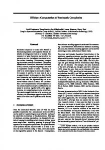
4.3 Computing Trade-Off Skylines To showcase the effect of trade-offs on the skyline size reduction, as well as the practical run-times, we actually computed some trade-off skylines using two typical real world datasets. Our real

world sets are genuine E-commerce data crawled in August 2009 and contain 998 notebook offers (http://www.shopping.com) and 1,350 real estate offers from the German city of Hamburg (http://www.immobilienscout24.de), respectively. The following evaluations can only be of a qualitative nature as trade-offs need to be semantically meaningful within their domain in order to be effective. In contrast arbitrarily chosen trade-offs (like used for the quantitative measurements) will rarely have useful effects on the actual skyline size. As the problem of suggesting and eliciting suitable trade-offs (see e.g. recent work on example critiquing) is beyond the scope of this work, we simply show that by even using very basic and straightforward heuristics, already significant reductions in skyline size are possible. The base idea of most trade-off suggestion algorithms is to reduce incomparability induced by a high degree of anti-correlation between two attributes and their respective correlated attributes. Consider our notebook dataset which features the following six numerical attributes: CPU speed, ram capacity, hard drive capacity, screen size, weight, and price. Based on the data, trade-offs can be straightforwardly suggested as follows: First, the two attributes with the strongest degree of anti-correlation are determined and their respective domain values are clustered. The attribute which shows clusters with a higher degree of separation and inner cohesion is selected as main attribute. Then the centroid values of the larger clusters form the base of one half of the suggested tradeoffs, e.g. for notebooks the main attribute is screen size with 15”, 14.1”, 13.3”, etc as clusters. These trade-offs‟ components are then expanded by the cluster‟s average values of all attributes which are correlated or anti-correlated with the main attribute, e.g. correlation coefficient ρ≥0.5 or ρ≤-0.5. For notebooks, these attributes are main memory, cpu speed, and weight, resulting in trade-off parts representing average 15”, 14.1”, and 13.3” with respect to the selected attributes, e.g. (15”, 3203 MB, 2082 MHz, 2.7 kg). Depending on the current scenario, two of these trade-off fragments are composed to a trade-off. 250 200

205 176

150 81

100

Skyline 57

50

T-Skyline

0 Notebooks

Real Estate

tion while the second part is improved by ¾ of the respective deviation. This result for example in the following trade-off typical for current mobile office laptops: 15”, 2302 MB, 1980 MHz, 2.9 kg) ⊳ 13.3”, 3909 MB, 2297 MHz, 1.71 kg . Incorporating two such trade-offs decreased the skyline size on average already by 15% to 176 items (see Figure 17). The resulting trade-off skylines also show a higher degree of focus, e.g. if emphasis is given on 15” notebooks, sub-par smaller or larger notebooks are removed if there is a corresponding good 15” notebook. However, in contrast to strict filtering, the Pareto characteristics are still maintained, e.g. sub-par 13.3” notebooks are only removed if a corresponding good 15” notebook exists; any outstanding 13.3” notebook will still remain in the skyline. We then did the same for the crawled real estate dataset. Again starting with the attribute pair showing the highest degree of anticorrelation, a trade-off was elicited. In this case the trade-off focused on space vs. price and we focused on rather spacey apartments and thus the trade-off can be relied on to remove average small-sized, but inexpensive apartments. For the real estate dataset originally consisting of 1350 items, the initial skyline set had still 81 items. When only integrating two trade-offs with respect to space and price this on average was already decreased by 30% (see Figure 17). On this practical data also the computation performance is very high. For the notebook dataset the computation of the initial skyline took 4 ms using an optimized block-nested loop implementation, while the trade-off skyline consumed additional 42 ms on average. For the real estate data set, the respective values are 3 ms and 12 ms. Of course we also wanted to investigate how the runtime performance of our algorithms scale for larger collections. Thus, we used a database of 50.000 items (which is already rather extensive for e-shopping portals). For the performance measurement we integrated up to 10 (again randomly chosen) trade-offs in a skyline query and calculated the respective results. The runtime results are presented in figure 18. All three algorithms (naïve baseline, 1-way indexing, and 2-way indexing) have been used with subsumption check. We can see that due to the non-indexed baseline is entirely out of scope starting at 3 seconds for only 2 trade-off, and quickly deteriorating (more than 3 minutes for 10 trade-offs). In contrast, the indexed version perform much better and even for 10 trade-off stay in the range of only a few seconds (including the time to build the index). Again we can see that the 2-way indexing clearly outperforms the 1-way indexing. Overall, these experiments show the practical applicability of trade-off skylines in real world scenarios like e.g., e-shopping. 14

Figure 17. Decrease of skyline size after integrating only two trade-offs runtime [sec]

For our notebook dataset of 998 items, the Pareto skyline still contains 205 items. Obviously still too many to process manually, and –as is the nature of skylines– also far too diverse. Thus, assume for example that a user intends to buy a mobile office laptop for writing papers on the road. Then a 15” screen size might be optimal for a given user while larger or smaller screens are less desirable. This information can be used to generate several tradeoffs, e.g. ((15", cluster avg. values) ⊳ 13.3”, cluster avg. values)), ((15", cluster avg. values) ⊳ (17", cluster avg. values)), etc. In order to express a further emphasis on the preferred cluster, the average values of the first part of the trade-off are slightly shifted in the less desired direction by ¾ of their standard devia-

12 10 8

NH

6

1-I

4

2-I

2 0 2

4

6

8

10

number of trade-offs in T

Figure 18. Runtime for integrating random trade-off into an independent dataset with 𝒅 = 𝟔 and 𝒏 = 𝟓𝟎, 𝟎𝟎𝟎

5. SUMMARY & OUTLOOK In this work we extended the well-established skyline paradigm with the concept of trade-offs, which allow for compensation between individual attribute dimensions in a qualitative fashion. Compensating (or trading) between different choices is indeed a very natural concept, frequently encountered in every days‟ decision processes. Trade-offs help to increase the focus and manageability of skylines without any arbitrary assumptions beyond the control of the user. However, up until now it was not possible to augment the strict Pareto semantics of traditional skylines with the compensating semantics of trade-offs. This is mainly caused by the fact that trade-offs break the convenient property of seperability when performing object domination tests, an integral component within any existing skyline algorithm. In this paper, we introduced the formal notion of trade-off skylines and designed the first trade-off skyline algorithm. We developed the object domination test criterion for skyline computation with respect to trade-offs. After establishing the formal properties, we derived a baseline trade-off algorithm which refines a given Pareto skyline with additional trade-off semantics. But in contrast to this baseline, our final algorithm does not rely on the exponential materialization of the full product order. To improve the performance, we showcased a tree data structure 𝑇𝑇𝑟𝑒𝑒 containing all necessary trade-off sequences to decide whether two objects dominate each other or not. This data structures especially paid attention to avoiding the storage of redundant information, thus saving storage space and computation time. In fact, it increases performance roughly by the factor of one order of magnitude over the baseline. Furthermore, we introduced an efficient two indexing scheme for the 𝑇𝑇𝑟𝑒𝑒 structure providing an additional performance boost by roughly the factor of 50 over the impractical baseline. Finally, a qualitative investigation of the skyline size reduction, and runtime measurements confirmed the benefits and practical applicability of our approach in real world scenarios like e.g., e-shopping. After establishing the theoretical foundations for trade-off skylines in this work, our future focus will be twofold: on one hand, the psychological aspects of the user interaction with trade-off skylines need to be examined, e.g., how should effective tradeoffs be elicited? Can trade-offs be suggested to the user in a semantically meaningful way? Which kinds of interfaces are suitable, which are not? How strongly are skylines focused by considering trade-offs, how do they affect the manageability of the result sets and thus helping the user to satisfy his/her information requirements? On the other hand, also technical performance improvements of the algorithm remain an issue for future exploration. These will cover further tuning of the algorithms, spanning from more efficient generation schemes or compressed storage of the sequences, to more efficient indexing allowing for faster object domination tests.

6. ACKNOWLEDGMENTS Part of this work was supported by a grant of the German Research Foundation (DFG) within the Emmy Noether Program of Excellence.

7. REFERENCES [1] Balke, W.-T., Lofi, C., Güntzer, U. Incremental Trade-Off Management for Preference Based Queries, Int. Jour. of Computer Science & Applications (IJCSA), 4 (Jun. 2007).

[2] Balke, W.-T., Zheng, J., Güntzer, U. Approaching the Efficient Frontier: Cooperative Database Retrieval Using HighDimensional Skylines, Conf. on Database Systems for Advanced Applications (DASFAA), Beijing, China, 2005. [3] Börzsönyi, S., Kossmann, D., Stocker, K. The Skyline Operator. Int. Conf. on Data Engineering (ICDE), Heidelberg, Germany, 2001. [4] Chan, C.-Y., Jagadish, H.V., Tan, K.-L., Tung, A. K. H., Zhang, Z. Finding k-dominant skylines in high dimensional space, Int. Conf. on Management of Data (SIGMOD), Chicago, IL, USA, 2006. [5] Chan, C.-Y., Jagadish, H.V., Tan, K.-L., Tung, A. K. H., Zhang, Z. On High Dimensional Skylines, Advances in Database Technology (EDBT), Munich, Germany, 2006. [6] Chomicki, J. Iterative Modification and Incremental Evaluation of Preference Queries. Int. Symp. on Found. of Inf. and Knowledge Systems (FoIKS), Budapest, Hungary, 2006. [7] Godfrey, P. Skyline cardinality for relational processing. How many vectors are maximal? Int. Symp. on Foundations of Information and Knowledge Systems (FoIKS). Vienna, Austria, 2004. [8] Godfrey, P.; Shipley, R.; Gryz. J. Maximal Vector Computation in Large Data. Int. Conf. on Very Large Databases (VLDB), Trondheim, Norway, 2005. [9] Hansson, S.O. Preference Logic, Handbook of Philosophical Logic, Second Edition, 4 (2002) [10] Ihab F. Ilyas and George Beskales and Mohamed A. Soliman. A Survey of Top-K Query Processing Techniques in Relational Database Systems, ACM Computing Surveys, 404 (2008) [11] Kossmann, D., Ramsak, F., Rost, S. Shooting Stars in the Sky: An Online Algorithm for Skyline Queries. Int. Conf. on Very Large Data Bases (VLDB), Hong Kong, China, 2002. [12] Lacroix, M., Lavency., P., Preferences: Putting more Knowledge into Queries. In.t Conf. Very Large Databases (VLDB), Brighton, UK, 1987. [13] Lee, J., You, G., Hwang, S. Telescope: Zooming to Interesting Skylines. Int. Conf. on Database Systems for Advanced Applications (DASFAA), Bangkok, Thailand, 2007. [14] Lofi, C., Balke, W.-T., Güntzer, U. Efficiently Performing Consistency Checks for Multi-Dimensional Preference Trade-Offs, Int. Conf. on Research Challenges in Computer Science (RCIS), Marrakech, Morocco, 2008. [15] Papadias, D., Tao, Y., Fu, G., Seeger, B. An Optimal and Progressive Algorithm for Skyline Queries. Int. Conf. on Management of Data (SIGMOD), San Diego, USA, 2003. [16] Pei, J., Jin, W., Ester, M., Tao, Y. Catching the best views of skyline: a semantic approach based on decisive subspaces. Int. Conf. on Very Large Data Bases, Trondheim, Norway, 2005 [17] Yuan, Y., Lin, X., Liu, Q., Wang, W.,Yu, J.Y., Zhang, Q., Efficient computation of the skyline cube, Int. Conf. on Very Large Data Bases, Trondheim, Norway, 2005.