52
JOURNAL OF SOFTWARE, VOL. 2, NO. 5, NOVEMBER 2007
Efficient Evaluation of Multiple-Output Boolean Functions in Embedded Software or Firmware Vaclav Dvorak Brno University of Technology, Brno, Czech Republic Email:
[email protected]
Abstract — The paper addresses software and firmware implementation of multiple-output Boolean functions based on cascades of Look-Up Tables (LUTs). A LUT cascade is described as a means of compact representation of a large class of sparse Boolean functions, evaluation of which then reduces to multiple indirect memory accesses. The method is compared to a technique of direct PLA emulation and is illustrated on examples. A specialized micro-engine is proposed for even faster evaluation than is possible with universal microprocessors. The presented method is flexible in making trade-offs between performance and memory footprint and may be useful for embedded applications where the processing speed is not critical. Evaluation may run on various CPUs and DSP cores or slightly faster on FPGA-based micro-programmed controllers. Index Terms — Embedded software, Boolean function evaluation, Binary Decision Diagrams, LUT cascades
I. INTRODUCTION Efficient evaluation of Boolean functions is an important part of many embedded software systems. Functions most frequently used in embedded system practice are not random, but application-specific with low complexity. Among them sparse functions defined below include applications such as encryption, data compression and conversion, pattern matching and searching, moving window functions on data streams, etc. We will address Boolean functions of large numbers (tens, hundreds) of variables because small size systems can be implemented directly in hardware, e.g. in PLA, ROM or TCAM (Ternary Content Addressable Memory). Software implementation of Boolean functions will be assumed in a form of a data structure describing the function and of a compiled program that reads the input vector and evaluates the function with the use of this data structure. The size of the code and of the data structure is one figure of merit and the other is the evaluation time from reading the input to generating the output. Hereafter we will use three compact representations: a PLA-like table, Look-Up Tables (LUTs) and binary decision diagrams (BDDs). The BDDs are well known, especially the reduced ordered BDDs (ROBDDs), [1]. On Based on “Time- and Space-Efficient Evaluation of Sparse Boolean Functions in Embedded Software”, by Vaclav Dvorak, which appeared in the Proceedings of the 14th IEEE Int. Conf. and Workshops on the Engineering of Computer-Based Systems 2007, Tuscon, AZ, USA, March 2007. © 2007 IEEE.
© 2007 ACADEMY PUBLISHER
the base of ROBDDs we will develop a more practical representation – cascades of LUTs. Software implementation of Boolean functions has been up to now studied especially in connection with PLCs (“ladder diagrams”) [2], digital system simulation, formal verification and testing [1], or specialized event processing [3], where either a speed (PLC) or a required memory were not that important. On the contrary, in embedded systems we do care for performance, memory space as well as for power consumption. We will demonstrate that presently used algorithms (PLA emulation, a BDD traversal or evaluation of Boolean expressions) are generally too slow and that the use of LUT cascades enables faster evaluation. The longer cascades with simpler LUTs are slower than shorter cascades with larger LUTs, and thus the processing speed can be even adjusted to requirements. The paper is structured as follows. In the following Section II we introduce terminology and notation concerning Boolean functions; a traditional approach to Boolean function evaluation is assessed in Section III. Binary decision diagrams (BDDs) and LUT cascades are introduced in Section IV, together with some complexity issues. Variable ordering in MTBDDs and in LUT cascades is a subject of Section V. In Section VI we give examples of LUT cascades for sample Boolean functions and illustrate trade-offs between speed of evaluation and required memory space. A micro-engine for LUT cascade processing is presented in Section VII. Results obtained with selected functions and some generalizations are commented on in Conclusions. II. TERMINOLOGY AND NOTATION To begin our discussion, we define the following terminology. A system of m Boolean functions of n Boolean variables, fn(i) : (Z2) n → Z2 , i = 1, 2, ..., m (1) will be simply referred to as multiple-output Boolean function Fn with output values from ZR = {0, 1, 2, …, R-1}, Fn: (Z2) n → ZR , (2) where R is the number of distinct combinations of m output binary values enumerated by values from ZR. Function Fn is incomplete if it is defined only on set X ⊂ (Z2) n; (Z2) n \ X = D is the don’t care set. The behavior of a combinational circuit can be described by the system of m explicit complete functions
JOURNAL OF SOFTWARE, VOL. 2, NO. 5, NOVEMBER 2007
© 2007 ACADEMY PUBLISHER
means of auxiliary variables. The advantage of the BDDs for CF is that tools useful for optimization of BDD for a single Boolean function (4) can be used without modification for multiple-output functions as well. As the LUT cascades are the main concern of this paper, we will provide a formal definition. A LUT will be also interchangeably referred to as a “cell”. Def. 1. A cascade C of a form k × m is the system C = [ K, M, H1, H2, …, HB, µ] where K ≤ 2k (M ≤ 2m) is the number of specified Boolean input vectors at k horizontal (m vertical) cell inputs, Hi: (Z2)k × (Z2)m → (Z2)k, 1 ≤ i ≤ B are functions implemented by individual cells, B, the cascade length, is the total number of cells and µ: {1,2,…, B}→(Z2)m assigns m-tuples of input variables xi , i = 1,2,…, n to B cells in the cascade. The above cascade has the width k horizontal rails carrying Boolean values and each cell has m vertical (side) inputs. The last cell in the cascade may have r ≠ k outputs. Def. 2. A cascade is said to be non-redundant if each variable used at vertical input enters one and only one cell. Otherwise the cascade is redundant. If a reference is made to a cascade, we will assume implicitly a nonredundant cascade. The attribute “redundant” will be used always explicitly. Note. Cascades considered in [16] use cells with additional vertical outputs. These intermediate outputs can reduce the cascade width k. Intermediate outputs are either individual Boolean variables yi as in (3) or the complete integer values from ZR as in (2); in the latter case BDD leaves appear not only in the bottom of the diagram, but span more its levels. A consequence for software evaluation is that some partial Boolean outputs or function values are generated earlier than others. III. TRADITIONAL APPROACHES TO EVALUATION OF BOOLEAN FUNCTIONS: PLA EMULATION Hardware implementation of Boolean functions in Programmable Logic Array (PLA) can serve as an initial prototype for software implementation. PLA consists of AND-matrix and OR-matrix. Rows of the AND-matrix define terms and OR-matrix serves for accumulation some of them into the binary outputs, Fig.1. AND array
OR array
n inputs
r outputs
p terms
of n variables yi = fn(i)(x1 , x2 , …, xn), i = 1, 2, ..., m (3) or y = F(x) in vector notation. Alternative implicit description is based on the so called output characteristic function (CF) [7] φ0 (x, y) = 1. (4) Machine representation of Boolean functions uses binary decision diagrams (BDDs), which can have many forms. Bit-level binary decision diagrams (BDDs), ordered binary decision diagrams (OBDDs) and reduced ordered binary decision diagrams (ROBDDs) are well known representation of a single Boolean function in a form of a directed acyclic graph [1]. Whereas ROBDD is a canonical (unique) representation for any given complete function and an order of variables, incomplete Boolean functions may be transformed into more than one complete form and into the associated ROBDD. Important parameters of a BDD are its size and width, i.e. the total number of decision nodes and the maximum number of edges between adjacent levels, where the edges pointing to the same nodes are counted as one. The size determines the memory space needed to store the BDD data structure while the width K (also C-measure, [4]) determines a BDD form factor since the height is given by the number of variables. The construction of minimum-size or by the same token minimum-width ROBDDs belong among NP-complete problems [5]; the size and width of the ROBDD depend on variable ordering and there are n! possible orderings of n variables. A heuristic approach can be used in a search for near-optimal orderings [6]. Upper bounds on the OBDD’s size and width for general random complete Boolean functions grow exponentially with number of variables n for any ordering, but functions used in digital systems design with few exceptions do have a reasonable BDD size and small width. M-ary decision diagrams are straightforward generalization of BDDs. They have two types of nodes: decision and terminal nodes. Decision node L is testing M-ary variable var(L) and its outgoing edges are marked by its values 0, 1, …, M-1. The terminal node assigns a single value from ZM (generally ZR, R≠M) to output y = Fn(x1, x2,…, xn). To represent a system of Boolean functions (1) by means of decision diagrams, we can use either m bit-level BDDs, one for each of m Boolean functions (possibly sharing some of their sub-diagrams in Shared BDDs or SBDDs, [7]), or one word-level BDD (WLBDD) with n Boolean decision variables and with R integer terminal values. There are many types of WLDDs. Multi-terminal BDDs have integer leaves and therefore represent functions from Booleans to integers. A BMD (Binary Moment Diagram) is more compact representation for some useful arithmetic functions which have exponential size if represented by MTBDDs. Hybrid decision diagrams HDDs are a combination of MTBDDs and BMDs. BDD for Characteristic Function (BDD for CF) [7] is yet another representation of multiple-output functions, which uses the shortest encoding of output vectors y by
53
Fig.1. Structure of PLA
54
JOURNAL OF SOFTWARE, VOL. 2, NO. 5, NOVEMBER 2007
The set of p terms produced by AND-matrix (a term vector) can be generated in parallel, each term in one bit of the computer word. If the capacity w bits in a single word is not enough, p/w computer words can be used to accommodate all the terms. The terms are evaluated in n steps, one input Boolean variable at a time. Two masks m0(x) and m1(x) of length p bits are maintained for each variable x. The masking bit of mask mv(x), v = 0,1, in a position of term t is denoted mv(x, t) and has the following value: if x occurs in t, then mv(x, t) = v if !x occurs in t, then mv(x, t) = !v if x does not occur in t, mv(x, t) = 1. Two masks for each variable are generated only once, at the beginning, based on their occurrence in PLA terms. The term vector is initialized to all ones and then a sequence of masks is applied to it using the bitwise logical AND operation. For variable x mask mv(x) is used depending on the input value x = v. All the terms are thus updated in parallel by the bitwise AND operation and the (full) width of computer word is utilized. As soon as all terms are ready, we have to emulate OR-matrix – apply bitwise OR operation selectively to certain bits. Another set of r masks will be used for r outputs. Unused terms in the term vector are masked out and if at least a single 1 remains, the result TRUE. The memory size for storing all sets of masks is thus space = (2n + r) p/w words (5) and time complexity is time = C1n + C2 r, (6) where C1 and C2 are execution times in clock cycles related to mask applications. If the number of terms p is less than the number of variables n, a dual evaluation method may be more advantageous. The relevant terms are generated one after another from the input vector using again two sets of masks. As soon as the term vector is assembled, the outputs are generated the same way as before. Similarly, if p < r, we can create the output vector faster by ORing p partial vectors mv(t); partial vector mv(t), v = 0,1, is selected if term t = v. Space and time complexities under all conditions are: 2n p / w r p / w space = + 2 p n / w 2 p r / w C n C r time = 1 + 2 C3 p C4 p p ≥ n p ≥ r conditions : + p < n p < r
Example: Size of full tables for two sample PLAs is given: TABLE 1. PARAMETERS OF PLA1 AND PLA2
PLA1 PLA2
n 13 11
r 8 8
© 2007 ACADEMY PUBLISHER
p 31 53
|X| 175 632
size [B] 8192 2048
Data structures for emulation of two PLAs with w = 8 bits according to (5) take up only 156 and 268 bytes, respectively. Time complexity is n + r = 21 and 19 time steps provided that C1 ≈ C2. (End of example.) IV. LUT CASCADES, BDDS AND COMPLEXITY ISSUES A. Relation of MTBDDs and LUT Cascades Whereas BDDs and MTBDDs proved useful in many areas of digital design [8] where they provide compact data structures and a degree of flexibility in manipulating them, they are not as wonderful for the purpose of function evaluation. The primary reason is the slow speed, since the evaluation process inspects one Boolean variable after another. There is though a certain speedup in comparison to direct evaluation of Boolean expressions, because each variable is processed only once. Straightforward remedy how to speed up the traversal of a BDD is to process several variables at a time. This way we will derive LUT cascades, in fact a special case of LUT networks. A close relation between both these representations of multiple-output Boolean functions will be illustrated on a n bit-counting example. The function Fn: Z2 → Zn counts the number of 1´s presented at n inputs and represents it by a binary number. The MTBDD and associated LUT cascade are displayed in Fig. 2 for n = 4. Generalization for larger values of n is easy. As the number of nodes grows linearly from the root to leaves, the width of the MTBDD is given by the last level of decision nodes and has the value of K = n. d c 0 b 0
0
1 c 1 b
0 1
a
c 2 b a
a 2
b 3
2
a 1
d
3
a 4
Fig.2. Bit counting example
(7) (8)
What connects two representations is the concept of sub-functions. Informally, the sub-function f of Fn is a function of s variables obtained from Fn by setting n− s variables to fixed constant values. The number of distinct sub-functions of s variables, s = 1, 2,…, n-1, the so called profile, characterizes complexity of the Boolean function. In Fig.2 we can recognize distinct sub-functions as edges crossing boundaries between MTBDD layers, counting edges incident with the same node only once. Edges are labeled by ID codes of distinct sub-functions. From the top down, there are 2 sub-functions of variables a, b, c (ID codes 0, 1), 3 sub-functions of variables a, b (ID codes 0, 1, 2), 4 sub-functions of variable a (ID codes 0, 1, 2, 3), and 5 sub-functions of zero variables (constant terminal values 0 to 4). LUT contents are defined by binary ID codes and a side variable entering a cell, and
JOURNAL OF SOFTWARE, VOL. 2, NO. 5, NOVEMBER 2007
binary ID codes generated by the cell. Co-synthesis of MTBDD and LUT cascade will be presented in Section V. As can be seen, the difference between the MTBDD and the LUT cascade is in communication among the MTBDD layers and LUTs in the cascade: in MTBDD each sub-function ID code requires an individual edge (”wire”), whereas the ID codes being sent between LUTs are binary coded. The number of rails k in the cascade is therefore k = log2 K. (9) This difference of two representations reflects itself in the way how the program interprets a certain applicationspecific MTBDD or a LUT cascade. In case of the MTBDD we may use for each node a record with 3 fields. A format indicator is one-bit field specifying the leaf node (leaf nodes may generally occur at any level of the diagram). Two other fields of the leaf node are then used for output. If the node is not a leaf, two fields (adjacent words) contain pointers to the base addresses of other nodes. The base address is then modified by the value of a current control variable(s) and is used to extract the correct field with the pointer to the next node. The program traverses a certain path in the MTBDD from the root to a leaf in at most n steps. LUTs are interpreted similarly, only the pointer to the next LUT is obtained from the current output by concatenating it with the control variable value and adding it up to the next LUT base address. If suitable, some LUTs can be combined to provide even faster processing (see first three cells in Fig.2 combined into one). B. Complexity isues Many questions arise in connection with implementation of the given multiple-output Boolean functions by LUT cascades. In our bit-counting example the number of sub-functions from the root to leaves (a profile) was increasing linearly. Some other functions may have a profile almost constant, what makes the number of rails in the cascade also constant – a desirable feature. However, for randomly generated functions and for multipliers the profile and maximum BDD width K increases exponentially (parameter k = log2 K linearly) with the number of variables. The question is, what will be the required number of cascade rails in general case. If we remove the restriction that each input variable can be used only once, the result is available as Theorem 1 for multi-valued redundant cascades (repeated BDDs): Theorem 1. [9] Every function Fn: (ZM) n → ZR, M ≥ 2, R > 2 is realizable by the LUT cascade with Bn cells (with Kvalued signals between adjacent cells and external Mvalued signals on side inputs). If R = 3, 4, 5, 7, 8, 9, 11, … then K = R else if R = 2, 6, 10,…, 2(2t+1), …, then K= R+1; (t=0,1,2,..). Bn= M(Bn-1 +1), B1=1. Synthesis method based on Theorem 1 is not practical, as it produces too long cascades and of the same length for functions with different complexity. However,
© 2007 ACADEMY PUBLISHER
55
redundant use of variables may sometimes be useful to reduce the number of cascade rails. Some examples are given in [11]. The size of the ROBDD for a single Boolean function of n variables given by Boolean expression in DNF is known to be less than the number of literals in the expression. More accurately is the BDD size upperbounded by [10] (10) P ≤ min L − k Ln + 2 k − 1 , k = 1,2,..., L, k
{
}
where L is the number of literals in DNF. Complexity of MTBDDs for general multiple-output Boolean functions gives the following Theorem 2 [11]: Size P and width K of the MTBDD for function Fn: (Z2) n → ZR are upper-bounded by i P ≤ min (2 n −i + R 2 ) − R − 1 i (11)
[
K ≤ max min( R 2 , 2 n−i ) i
i
]
The width K of MTBDD and thus the cascade width k (a number of rails) have reasonably low values for many functions arising in practice. One class of such functions is defined below. Def. 3. Sparse functions. Under the sparse functions Fn: (Z2)n → ZR we will understand functions with the domain (Z2)n divided into n two parts X and D, (Z2)n = X ∪ D, | X |