Efficient Method for Optimizing Artificial Neural

Volume 4, Issue 6, June 2014

ISSN: 2277 128X

International Journal of Advanced Research in Computer Science and Software Engineering Research Paper Available online at: www.ijarcsse.com

Efficient Method for Optimizing Artificial Neural Network Using „Quantum-Based Algorithm‟ Mr. Avinash Jagtap 1 ( ME IT Student) Siddhant College of Engineering, University of Pune, India

Prof. Rashmi Deshpande 2 (Assistant Professor) Siddhant College of Engineering University of Pune, India

ABSTRACT- This paper presents competent Method for Optimizing Artificial Neural Network Using Quantum Based Algorithm. In the evolutionary process, the Quantum bits refined so that the probability of finding the optimal network is increased. The probability representation reduced the non positive impact of the permutation problem and the risk of the potential network. To finds near-optimal connection weights, the technique of subspace search using quantum bits is proposed. The algorithm thus performed a division-by-division exploration in the beginning and, as the candidate subspaces are identified, a randomized search in good subspaces is employed for exploitation. This is helpful to provide a set of appropriate weights when evolving the network structure and to alleviate the noisy fitness evaluation problem. The Propose model Improved QNN performance better than standard QNN based on some bench test function. Application examples on iris and breast cancer are shown the Improved QNN performance better than standard QNN based. KEYWORDS: Quantum neural network, mapping problem, classification, learning structure. I. INTRODUCTION ARTIFICIAL neural networks (ANNs) used in many areas, such as modeling [1], prediction [2], classification [3], and pattern recognition [4]. Neural network was proved to be a universal approximation [5].Neural networks are widely applied in areas such as prediction In general, too large a network may tend to over fit the training data and affect the generalization capability, whereas too small a network may not even be able to learn the training samples due to its limited the representation capability. In addition, a fixed structure of overall connectivity between neurons may not provide the optimal performance within given training period [6]. Therefore, recently, some Attention has been given to the problem of how to construct a suitable network structure for a given task. With little or no prior knowledge about the problem, on usually determines the network structure by means of a trial and- error procedure. However, this depends heavily on the user experience and may require intensive human interaction and computational time. Research has been conducted on constructive algorithms [9], [10] (i.e., start with the smallest possible network and gradually add neurons or connections) and destructive algorithms [11], [12] (i.e., start with the largest Possible network and delete unnecessary neurons and connections) to aid the automatic design of structures. However, as indicated in [13], the structural hill-climbing methods in these algorithms are susceptible to being trapped at structural local optima. The search of the optimal network structure is known to be a complex, non differentiable, and multi modal optimization problem, making evolutionary algorithms (EAs) a better candidate for the task than the constructive and destructive algorithms [14]. In the structure design, EAs are employed in two ways: to evolve the structures only [15] and to evolve both the structures and the connection weights simultaneously [13]. In general, when EAs are used to determine the structures only, the training error is calculated by performing a random initialization of weights, which are then determined by a learning algorithm such as a back propagation [16]. However, as indicated in [17], the training results depend on the random initial weights and the choice of learning algorithm. Hence, the same representation (genotype) of structure may have quite different levels of fitness. This one-to many mapping from genotype to the actual networks (phenotypes) may induce noisy fitness evaluation and misleading evolution. To obtain the network structure automatically, constructive and destructive algorithms can be used [18]. A small network may not provide good performance owing to its limited information processing power. A large network, on the other hand, may have some of its connections redundant [18], [19]. Moreover, the implementation cost for a large network is high. The parents, determining the mutations to be performed, and mutating the copy. The constructive algorithm starts with a small network. Hidden layers, nodes, and connections are added to expand the network dynamically [19]–[24]. The destructive algorithm starts with a large network. Hidden layers, nodes, and connections are then deleted to contract the © 2014, IJARCSSE All Rights Reserved

Page | 692

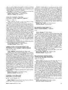
Jagtap et al., International Journal of Advanced Research in Computer Science and Software Engineering 4(6), June - 2014, pp. 692-700 network dynamically [25], [26]. The design of a network structure can be formulated into a search problem. GAs [27], [28] were employed to obtain the solution. Pattern classification approaches [29] can also be found to design the network structure. Some other methods were proposed to learn both the network structure and connection weights. to solve this problem we developed the QNN and this QNN gives better result than the other algorithm. II. RELATED WORK The QNN has distinct advantages over general EAs when it is used in evolving the networks. First, each individual in the QNN is composed of quantum bits that represent the probability of good connections and weight subspaces rather than a specific structure and weight values. So, if the network has bad fitness owing to the one-to-many or many-to-one mapping problem, QNN modifies the quantum states rather than discarding this network. Thus, the risk of throwing away a potential structure or weight values is mitigated. Second, instead of the crossover and mutation, the QNN uses observation to create a new network. Thus, the negative impact of the permutation problem is reduced. Third, a partitioning strategy is used to find the near-optimal connection weights. It explores each weight space section-by-section and rapidly finds the promising subspace for further exploitation. This is helpful to provide a set of appropriate weights when evolving the network structure and alleviate the noisy fitness evaluation problem the output of neural network is processed by applying before thresholding parameters to predict the classification so it gives improved performance than the standard QNN. III. QNN Architecture (A) QNN Architecture Network basic network considered in this paper is a generalized MLP (GMLP) network, which consists of an input layer, an output layer, a number of hidden nodes, and associated interconnections. Let X and Y be the input and output vectors, respectively. The GMLP network with m inputs, nh hidden nodes, and n outputs is characterized by the equations xi = Xi, 1≤i m xi =



i 1 j 1

wijxj m ≤ i ≤ m +nh+ n

Yi=xi+m+nh 1≤i≤m (1) where wij is the weight of the connection from node j to node i and f is the sigmoid function (2) f ( z )  1 z 1 e

Cmax = m (nh+ n) +

((nh + n)(nh + n - 1 ) ) 2

(3)

Fig 1.GMLP Where the first term on the right-hand side is related to the number of connections from the input nodes to the hidden and output nodes, and the second term is related to the number connections from the hidden nodes to the output nodes. Thereby, the selection of the appropriate network is equivalent to finding the optimal weighting vector s whose components are the weightings wij with maximum dimension. © 2014, IJARCSSE All Rights Reserved

Page | 693

Jagtap et al., International Journal of Advanced Research in Computer Science and Software Engineering 4(6), June - 2014, pp. 692-700 (B) Objective Function In this paper, the winner-takes-all classification rule is used; that is, the output with the highest activation determinates the class. The network error for the pattern t is defined as

e(t )  {10TifT^(^t ()t)T(Tt ()t )

(4)

Where Tˆ (t) and T (t) are the assigned class and the true class of the pattern t, respectively. The objective function F(s), which represents the percentage of incorrectly classified patterns, is

F (s) 

1 0  e(t ) D t 1

(5)

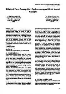
Where D is the number of patterns. The problem thus becomes the determination of the optimal s such that the objective function F(s) is minimized. (c) Representation of Solutions In this paper, quantum bits are employed to represent the probabilities of various network connectivity and connection weights. More precisely, in the QNN, each solution is composed of C, which contains a string of quantum bits that represent the network connectivity, and W, which contains the quantum bits that represent the connection weights. The vector C is expressed as C=Qc=α1|α2|…|αcmax (6) Where αi, i = 1, 2. . . Cmax is quantum bit. The connectivity vector C utilizes cmax quantum bits to represent the probabilities of 2cmax structures. The connection weight W is expressed as W=(Qw1,Qw2.Qwcmax) (7) where each Qwi, i = 1, 2, . . . , cmax, is assumed to contain k quantum bits Thus, each weight space is divided into 2k subspaces and Qwi is used to represent the probability of the subspaces that render good weight values. The specific realization associated with each quantum bit of the weighting is governed by a Gaussian random number generator with mean μi, j and variance (σi, j ), N(μi, j , σi, j ), where j = 1, 2, , ….2k.

i =1,2,… . ..Cmax j=1,2,……2𝐾 Fig 2 Step of QNN in the population © 2014, IJARCSSE All Rights Reserved

Page | 694

Jagtap et al., International Journal of Advanced Research in Computer Science and Software Engineering 4(6), June - 2014, pp. 692-700 IV. QUANTUM-BASED ALGORITHM 1) Initialize the population by specifying the quantum sets and of each individual and selecting the mean i, j and standard deviation i, j , where g =1, 2, . . . , G, l = 1, 2, . . . , L, i = 1, 2, . . . , cmax, and j = 1, 2, . . . , 2𝑘 . 2) Set generation as 1. 3) for each subpopulation g = 1, 2, . . . , G do 3.1) Observe Qc

(g)

to give a binary string bc.

*(g )

*(g )

3.2) If bc is empty, store bc as bc . 3.3) for each individual l = 1, 2, . . . , L do 3.3.1) for each weight i = 1, 2, . . . , cmax do If the i th bit in bc is 1 (i.e., the i th connection is present) then • Observe Qwi

( g ,l )

to give a binary string

bwi .

*(g ,l )

• If bwi is empty, store bwi as bwi*(g,l) subpopulation • Determine the j th subspace as a candidate subspace according to j = d (bwi) + 1. • Generate a weight value wi from N(i,j, i, j). end if end for 3.3.2) obtain a solution s and compute the objective function F(s). 3.4) If generation is 1, store argmin l∈ {1,2,...,L}F*(g,l) individualas F*(g)subpopulation. 3.5)If argminl∈ {1,2,...,L}F*(g,l)individual > F(g)subpopulation, update Q(g)c ; else update b(g)c and F(g)subpopulation. end for 4) If the termination condition is satisfied, go to Step 7. 5) If the exchange condition is satisfied, perform exchange operation. 6) Increment generation by 1 and return to Step 3. 7) Choose arg ming∈ {1,2,...,G}F*(g)subpopulation as the minimum objective function value and the corresponding s*(g,l) as the optimal solution.

V. NUMERICAL EXPERIMENTS AND RESULTS This section presents the QNNs performance for four well-known benchmark classification problems, namely breast cancer and iris, heart, and diabetes problems. These problems, from the University of California Irvine Machine Learning Repository, are widely used in studies on ANNs and machine learning [17], [30]. Detailed descriptions of these problems can be obtained from [31] and [32]. © 2014, IJARCSSE All Rights Reserved

Page | 695

Jagtap et al., International Journal of Advanced Research in Computer Science and Software Engineering 4(6), June - 2014, pp. 692-700 A. Experimental Setup In this paper, the data sets of each problem are divided into three sets: 50% for training, 25% for validation, and 25% for testing. The training set is used to train and modify the structure and weights of the ANN. The validation set is used to determine the final architecture from the well-trained individuals, and the testing set is used to measure its generalization ability. The parameters of the QNN shown in Table I are used for all the problems to show the robustness of the model regarding the parameter settings. Note that the number of the quantum bits in Qc is related to the maximum number of connections, which is determined by the number of inputs, outputs, and hidden nodes. The number of quantum bits in Qw (i.e., k) governs the partitioning of each weight space and affects the subspace size. A large number of quantum bits imply a small subspace size and a strong possibility of escaping from a local optimum. However, the computational complexity increases with the number of subspaces. In this paper, k is set to 4, which means that each weight space is divided into 24 subspaces. _θ affects the convergence speed of a quantum bit. Convergence may occur prematurely if this parameter is set too high. A value from 0.01π to 0.05π is recommended for the magnitude of _θ, although it depends on the problem. In the experiments, _θ was set to 0.05π. ε is applied to quantum bit αi to make the probability (αi)2converge to either ε or 1− ε rather than zero or unity. When (αi )2 converges to ε (or 1−ε), it means that the i th quantum bit will be found in state “1” with probability ε (or 1 − ε) and state “0” with probability 1 − ε (or ε). So, ε can be regarded as a mutation probability and should usually be set fairly low (0.005–0.01 is a good choice). If it is set too high,the search will turn into a primitive random search. In the experiments, ε was set to 0.005. τ is the multiplication factor that governs the convergence rate of the SD. Convergence may occur prematurely if this parameter is set too low. A value from 0.8 to 0.95 was found to be suitable. In the experiments, it was set to 0.8. The number of hidden nodes nh is manually chosen as 2, 3, 4, 5, 6, 7, 8, 10, 12, and 14 to test the learning performance (the cases of nh = 9, 11, and 13 are omitted to save space). For all experiments, the evolution is repeated until 2000 generations is reached. To assess the performance of the algorithm, 100 runs are conducted. In each run, the testing error of the best model in terms of the validation error is stored. The error rate and the number of connections, obtained by taking the average and the SD of the 100 records, are also computed. B. Experimental Results and Comparisons 1) Classification of the Iris Data Set: This data set contains three classes of 50 instances each (total number of instances is 150), where each class refers to a type of iris plant. One class is linearly separable from the other two, which are not linearly separable from each other. The number of attributes is four, all of which are real values. In the experiment, the data set items are randomly chosen with 90 instances for training, 15 instances for validation, and the rest (45 instances) for testing. Table II shows the classification results of the QNN for various numbers of hidden nodes (nh). As can be seen, the QNN achieves good training performance for almost all values of nh. A mean training error of 0 was obtained for nh = 2, 4, and 7. For the testing set, the best models in terms of validation error achieved a minimum testing error of 0 with all values of nh . Furthermore, the best mean testing error is 1.21%, and the nh corresponding average number of connections is 62.35 (the number of connections of a fully connected network is 130), which is approximately a 52% reduction in links. Although a direct comparison with other approaches is difficult because the algorithms and methods of obtaining the generalization of the models are different, it is interesting to compare the results in terms of testing error obtained in other publications. Table III shows the results from some existing approaches and the best result of the QNN in terms of the mean testing error in Table II. As can be seen, the QNN has the lowest mean testing error. In fact, the mean testing errors of the QNN for all values of nh are lower than those of the other models. This demonstrates the powerful classification ability of the QNN under various network sizes. 2) Classification of the Cancer Data Set: This data set contains patterns of 699 individuals. Each pattern has nine attributes and two classes. All the attributes are real values. The task is to classify a tumor as either benign or malignant based on cell descriptions gathered from a microscopic examination. In the experiment, the data are split into three sets: 350 samples in the training set, 175 samples in the validation set, and 174 samples in the testing set. The classification results of the QNN for various values of nh are shown in Table IV. As can be seen, the evolution for various values of nh has a considerably low variance in the error rate. For example, the mean training error is 2.89% when nh = 2,3 or 4, and the mean training errors are 2.90%, 2.91%, and 2.92% when nh = 5 or 7, nh = 6, 8, or 12, and nh = 10 or 14, respectively. This means that the QNN is robust regarding this parameter. More specifically, the value of nh affects the network size but it does not appear to affect the training ability of the QNN. Similar results were observed with the testing set. For the testing set, the best mean error is 0.89%, and the average number of connections is 105.85 (the number of connections of a fully connected network is 217), which is approximately a 51% reduction in links. Table V shows the results from some existing approaches and the best result of the QNN. As can be seen, the QNN has the lowest mean testing error. In addition, the mean testing errors for all values of nh are considerably lower than those of the other models, except for New Constructive Algorithm (NCA). Therefore, for the cancer data set, it can be concluded that the QNN is superior to or as good as many of the state-of-the-art models of evolutionary neural networks. VI. Improve ANN by introducing thresholding parameters: The output of neural network is processed by applying before thresholding parameters to predict the classification. Suppose we have iris data with class: 1, 2 & 3; if predicted class value between P1 < 1.5 -- After threshold classification number: 1if © 2014, IJARCSSE All Rights Reserved

Page | 696

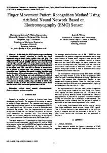
Jagtap et al., International Journal of Advanced Research in Computer Science and Software Engineering 4(6), June - 2014, pp. 692-700 predicted class value between 1.5 < P1 < 2.5 -- After threshold classification number: 2if predicted class value between 2.5 < P1 -- After threshold classification number: 3 improved ANN by changing Tau (Learning) parameter 1) if the fitness value < Optimum Sigma = Optimum Sigma * Tau *0.92) if the fitness value > Optimum Sigma = Optimum Sigma * Tau* 1.1 We have compared to existent data set of iris and breast cancer then we got 25% improved result. Actually we change the learning parameter and this parameter of tau was fix in the 0.8 in the existent system if we change this parameter plus and negative form then we got some variance data and this data gives better result [33]. Table II. PERFORMANCE OF THE QNN FOR THE IRIS DATA SET (ALL RESULTS WERE AVERAGED OVER 20 INDEPENDENT RUNS)

8

Iris

nh = 2 nh = 6 nh = 10

Training Error rate (%)

6 4 2 0 0

1

-2

2

3

4

5

6

7

Number of Quantum bits in (Qw)

Testing Error rate (%)

10

Iris

8

nh = 2

6

nh = 6

4 2 0 0

1

2 5 Number of3Quantum 4bits in (Qw)

6

7

Fig. 3 Training and testing error rates of the Iris problems with nh = 2, 6, 10, and 14 at k = 0, 1, 2, 3, 4, 5, and 6. © 2014, IJARCSSE All Rights Reserved

Page | 697

Jagtap et al., International Journal of Advanced Research in Computer Science and Software Engineering 4(6), June - 2014, pp. 692-700

Fig. 4 Training and testing error rates of the heart and diabetes problems with nh = 2, 6, 10, and 14 at k = 0, 1, 2, 3, 4, 5, and 6. TABLE III Comparisons of THE QNNs Results for the Iris Data set with Those obtained for other models in terms of average Testing MODEL Author Mean Testing Error (SD) (%) QNN 1.21(0.78) AMGA M. M. Islam et al. [33] 1.89(-) HMOEN_L2 C. K. Goh et al. [32] 2.00(1.84) NCA M. M. Islam et al. [33] 2.16(0.18) OMNN T.B.Ludermir et.al [20] 4.62(-) OC1-AP E. Cantú-Paz et al. [33] 6.10(0.5) HMOEN_HN C. K. Goh et al. [32] 3.74 (1.1) Table IV PERFORMANCE OF THE QNN FOR THE CANCER DATA SET (ALL RESULTS WERE AVERAGED OVER 20 INDEPENDENT RUNS)

© 2014, IJARCSSE All Rights Reserved

Page | 698

Jagtap et al., International Journal of Advanced Research in Computer Science and Software Engineering 4(6), June - 2014, pp. 692-700 TABLE V Comparisons of THE QNNs Results for the CANSER Data set with Those obtained for other models in terms of average Testing MODEL Author Mean Testing Error (SD) (%) QNN 0.89 (0.32) NCA M. M. Islam et al. [35] 0.91 (0.24) AMGA M. M. Islam et al. [33] 1.30 (-) HMOEN_HN SNG HMOEN_L2 CFNN OC1-AP

C. K. Goh et al. [32] N. Garcia-Pedrajas et al. [36] C. K. Goh et al. [33] L. Ma et al. [38] E. Cantú-Paz et al. [37]

3.18 (0.58) 2.78 (1.18) 3.74 (1.1) 3.30 (-) 5.30 (0.4)

VII. CONCLUSION The aim was to design an ANN with few connections and high classification performance by simultaneously optimizing the network structure and the connection weights. In addition, in the proposed model, each weight space is decomposed into subspaces in terms of quantum bits. Thus, the algorithm performs a region by region exploration, and evolves gradually to find promising subspaces for further exploitation. This was helpful to provide a set of appropriate weights when evolving the network structure and to alleviate the noisy fitness evaluation problem. An improved QNN has been proposed in this paper. By using the benchmark test functions, it has been shown that the improved QNN performs more efficiently than the standard QNN. Using the improved QNN, the proposed neural network is able to learn both the input– output relationship of an application and the network structure. As a result, a given fully connected neural network can be reduced to a partially connected network after learning. This implies that the cost of implementation of the neural network can be reduced. Application examples on Iris and breast cancer using the proposed neural network trained with the improved QNN have been given. ACKNOWLEDGMENT We would like to thank Prof. Rashmi Deshpande for her tremendous support. Also we would like to thanks Dept. Head Prof. S.A. Nalawade who always gave attention to help us in developing this project. This work is supported by Siddhant College of Engineering, Pune, India Year 2014. REFERENCES [1] R. Xuemei and L. Xiaohua, “Identification of extended Hammerstein systems using dynamic self-optimizing neural networks,” IEEE Trans. Neural Netw., vol. 22, no. 8, pp. 1169–1179, Aug. 2011. [2] P. K. Patra, M. Sahu, S. Mohapatra, and R. K. Samantray, “File access prediction using neural networks,” IEEE Trans. Neural Netw., vol. 21, no. 6, pp. 869–882, Jun. 2010. [3] T. H. Oong and N. A. M. Isa, “Adaptive evolutionary artificial neural networks for pattern classification,” IEEE Trans. Neural Netw., vol. 22, no. 11, pp. 1823–1836, Nov. 2011. [4] K. Jonghoon, L. Seongiun, and B. H. Cho, “Complementary cooperation algorithm based on DEKF combined with pattern recognition for SOC/capacity estimation and SOH prediction,” IEEE Trans. Power Electron., vol. 27, no. 1, pp. 436–451, Jan. 2012. [5] X. Yao, “Evolving artificial neural networks,” Proc. IEEE, vol. 87, no. 9, pp. 1423–1447, Sep. 1999. [6] S. Van den Dries and M. A. Wiering, “Neural-fitted TD-leaf learning for playing othello with structured neural networks,” IEEE Trans. Neural Netw. Learn. Syst., vol. 23, no. 11, pp. 1701–1713, Nov. 2012. [7] M. H. Shih and F. S. Tsai, “Decirculation process in neural network dynamics,” IEEE Trans. Neural Netw. Learn. Syst., vol. 23, no. 11, pp. 1677–1689, Nov. 2012. [8] C. Xiao, Z. Cai, Y. Wang, and X. Liu, “Tuning of the structure and parameters of a neural network using a good points set evolutionary strategy,” in Proc. 9th Int. Conf. Young Comput. Sci., Nov. 2008, pp. 1749–1754. [9] R. Parekh, J. Yang, and V. Honavar, “Constructive neural-network learning algorithms for pattern classification,” IEEE Trans. Neural Netw., vol. 11, no. 2, pp. 436–450, Mar. 2000. [10] M. M. Islam, X. Yao, and K. Murase, “A constructive algorithm for training cooperative neural network ensembles,” IEEE Trans. Neural Netw., vol. 14, no. 4, pp. 820–834, Jul. 2003. [11] H. H. Thodberg, “Improving generalization of neural networks through pruning,” Int. J. Neural Syst., vol. 1, no. 4, pp. 317–326, Jul. 1991. [12] R. Reed, “Pruning algorithms-a survey,” IEEE Trans. Neural Netw., vol. 4, no. 5, pp. 740–747, Sep. 1993. [13] P. J. Angeline, G. M. Sauders, and J. B. Pollack, “An evolutionary algorithm that constructs recurrent neural networks,” IEEE Trans. Neural Netw., vol. 5, no. 1, pp. 54–65, Jan. 1994. © 2014, IJARCSSE All Rights Reserved

Page | 699

[14] [15] [16]

[17] [18] [19] [20] [21]

[22] [23]

[24]

[25] [26] [27] [28] [29] [30] [31] [32] [33] [34] [35]

[36] [37] [38]

Jagtap et al., International Journal of Advanced Research in Computer Science and Software Engineering 4(6), June - 2014, pp. 692-700 G. F. Miller, P. M. Todd, and S. U. Hedge, “Designing neural networks,” Neural Netw., vol. 4, pp. 53–60, Nov. 1991. N. Nikolaev and H. Iba, “Learning polynomial feedforward neural networks by genetic programming and backpropagation,” IEEE Trans. Neural Netw., vol. 14, no. 2, pp. 337–350, Mar. 2003. D. E. Rumelhart, G. E. Hinton, and R. J. Williams, “Learning internal representations by error propagation,” in Parallel Distributed Processing, vol. 1, D. E. Rumelhart and J. L. McClelland, Eds. Cambridge, MA, USA: MIT Press, 1986, pp. 318–362. X. Yao and Y. Liu, “A new evolutionary system for evolving artificial neural networks,”IEEE Trans. Neural Netw., vol. 8, no. 3, pp. 694 713, May 1997. F. H. F. Leung, H. K. Lam, S. H. Ling, and P. K. S. Tam, “Tuning of the structure and parameters of a neural network using an improved genetic algorithm,” IEEE Trans. Neural Netw., vol. 14, no. 1, pp. 79–88, Jan. 2003. J. Tsai, J. Chou, and T. Liu, “Tuning the structure and parameters of a neural network by using hybrid Taguchigenetic algorithm,”IEEE Trans. Neural Netw., vol. 17, no. 1, pp. 69–80, Jan. 2006. T. B. Ludermir and C. Zanchettin,“An optimization methodology for neural network weights and architectures,” IEEE Trans. Neural Netw., vol. 17, no. 6, pp. 1452–1459, Nov. 2006. L. Li and B. Niu, “A hybrid evolutionary system for designing artificial neural networks,” in Proc. Int. Conf. Comput. Sci. Softw. Eng., vol. 4. Dec. 2008, pp. 859–862. R. K. Belew, J. McInerney, and N. N. Schraudolph, “Evolving networks: Using genetic algorithm with connectionist learning,” Dept. Comput. Sci. Eng., Univ. California, San Diego, CA, USA, Tech. Rep. CS90– 174, Feb. 1991. P. J. B. Hancock, “Genetic algorithms and permutation problems: A comparison of recombination operators for neural net structure specification,” in Proc. Int. Workshop Combinat. Genet. Algorithms Neural Netw., Jun. 1992, pp. 108–122. J. D. Schaffer, L. D. Whitley, and L. J. Eshelman, “Combinations of genetic algorithms and neural networks: A survey of the state of the art,” in Proc. Int. Workshop Combinat. Genet. Algorithms Neural Netw., Jun. 1992, pp. 1– 37. V. Maniezzo, “Genetic evolution of the topology and weight distribution of neural networks,” IEEE Trans. Neural Netw., vol. 5, no. 1, pp. 39–53, Jan. 1994. J. Fang and Y. Xi, “Neural network design based on evolutionary programming,” Artif. Intell. Eng., vol. 11, no. 2, pp. 155–161, Apr. 1997. X. Yao and Y. Liu, “Toward designing artificial neural networks by evolution,” Appl. Math. Comput., vol. 91, no. 1, pp. 83–90, Apr. 1998. P. Kohn, “Combining genetic algorithms and neural networks,” M.S. thesis, Dept. Comput. Sci., Univ. Tenessee, Knoxville, TN, USA, 1994. K. O. Stanley and R. Miikkulainen, “Evolving neural networks through augmenting topologies,” Evol. Comput., vol. 10, no. 2, pp. 99–127, G. Bebis, M. Georgiopoulos, and T. Kasparis, “Coupling weight eliminationwith genetic algorithms to reduce network size and preserve generalization,” Neurocomputing, vol. 17, pp. 167–194, May 1997. L. Prechelt, “PROBEN1-A set of neural network benchmark problems and benchmarking rules,” Faculty Informat., Univ. Karlsruhe, Karlsruhe, Germany, Tech. Rep. 21/94, Sep. 1994. C. K. Goh, E. J. Teoh, and K. C. Tan, “Hybrid multiobjective evolutionary design for artificial neural networks,” IEEE Trans. Neural Netw.,vol. 19, no. 9, pp. 1531–1548, Sep. 2008. M. M. Islam, M. A. Sattar, M. F. Amin, X. Yao, and K. Murase, “A new adaptive merging and growing algorithm for designing artificial neural networks,” IEEE Trans. Syst. Man Cybern., vol. 39, no. 3, pp. 705–722, Jun. 2009. Quantum-Based Algorithm for Optimizing Artificial Neural Networks Tzyy-Chyang Lu, Gwo-Ruey Yu, Member, IEEE, and Jyh-Ching Juang, Member, IEEE.VOL. 24, NO. 8, AUGUST 2013. M. M. Islam, M. A. Sattar, M. F. Amin, X. Yao, and K. Murase, “A new constructive algorithm for architectural and functional adaptation of artificial neural networks,” IEEE Trans. Syst. Man Cybern., vol. 39, no. 6, pp. 1590–1605, Dec. 2009. N. Garcia-Pedrajas, C. Hervas-Martinez, and D. Ortiz-Boyer, “Cooperative coevolution of artificial neural networks ensembles for pattern classification,” IEEE Trans. Evol. Comput., vol. 9, no. 3, pp. 271–302, Jun. 2005. E. Cantú-Paz and C. Kamath, “Inducing oblique decision trees with evolutionary algorithms,” IEEE Trans. Evol. Comput., vol. 7, no. 1, pp. 54–68, Feb. 2003. L. Ma and K. Khorasani, “Constructive feedforward neural networks using Hermite polynomial activation functions,” IEEE Trans. Neural Netw., vol. 16, no. 4, pp. 821–833, Jul. 2005.

© 2014, IJARCSSE All Rights Reserved

Page | 700