Efficient Non-Parametric Function Induction in Semi-Supervised

Efficient Non-Parametric Function Induction in Semi-Supervised Learning

Olivier Delalleau, Yoshua Bengio and Nicolas Le Roux Dept. IRO, Universit´e de Montr´eal P.O. Box 6128, Succ. Centre-Ville, Montreal, H3C 3J7, Qc, Canada {delallea,bengioy,lerouxni}@iro.umontreal.ca

Abstract There has been an increase of interest for semi-supervised learning recently, because of the many datasets with large amounts of unlabeled examples and only a few labeled ones. This paper follows up on proposed nonparametric algorithms which provide an estimated continuous label for the given unlabeled examples. First, it extends them to function induction algorithms that minimize a regularization criterion applied to an outof-sample example, and happen to have the form of Parzen windows regressors. This allows to predict test labels without solving again a linear system of dimension n (the number of unlabeled and labeled training examples), which can cost O(n3 ). Second, this function induction procedure gives rise to an efficient approximation of the training process, reducing the linear system to be solved to m  n unknowns, using only a subset of m examples. An improvement of O(n2 /m2 ) in time can thus be obtained. Comparative experiments are presented, showing the good performance of the induction formula and approximation algorithm.

1

INTRODUCTION

Several non-parametric approaches to semi-supervised learning (see (Seeger, 2001) for a review of semisupervised learning) have been recently introduced, e.g. in (Szummer & Jaakkola, 2002; Chapelle et al., 2003; Belkin & Niyogi, 2003; Zhu et al., 2003a; Zhu et al., 2003b; Zhou et al., 2004). They rely on weak implicit assumptions on the generating data distribution, e.g. smoothness of the target function with respect to a given notion of similarity between examples1 . For 1 See also (Kemp et al., 2004) for a hierarchically structured notion of a priori similarity.

classification tasks this amounts to assuming that the target function is constant within the region of input space (or “cluster” (Chapelle et al., 2003)) associated with a particular class. These previous non-parametric approaches exploit the idea of building and smoothing a graph in which each example is associated with a node, and arcs between two nodes are associated with the value of a similarity function applied on the corresponding two examples. It is not always clear with these graph-based kernel methods for semi-supervised learning how to generalize to previously unseen test examples. In general they have been designed for the transductive setting, in which the test examples must be provided before doing the expensive part of training. This typically requires solving a linear system with n equations and n parameters, where n is the number of labeled and unlabeled data. In a truly inductive setting where new examples are given one after the other and a prediction must be given after each example, it can be very computationally costly to solve such a system anew for each of these test examples. In (Zhu et al., 2003b) it is proposed to assign to the test case the label (or inferred label) of the nearest neighbor (NN) from the training set (labeled or unlabeled). In this paper we derive from the training criterion an inductive formula that turns out to have the form of a Parzen windows predictor, for a computational cost that is O(n). Besides being smoother than the NN-algorithm, this induction formula is consistent with the predicted labels on the unlabeled training data. In addition to providing a relatively cheap way of doing function induction, the proposed approach opens the door to efficient approximations even in the transductive setting. Since we know the analytic functional form of the prediction at a point x in terms of the predictions at a set of training points, we can use it to express all the predictions in terms of a small subset of m  n examples (i.e. a low-rank approximation) and solve a linear system with m variables and equations.

2

NON-PARAMETRIC SMOOTHNESS CRITERION

for i ∈ L ∪ U then gives rise to the linear system

In the mathematical formulations, we only consider here the case of binary classification. Each labeled example xk (1 ≤ k ≤ l) is associated with a label yk ∈ {−1, 1}, and we turn the classification task into a regression one by looking for the values of a function f on both labeled and unlabeled examples xi (1 ≤ i ≤ n), such that f (xi ) ∈ [−1, 1]. The predicted class of xi is thus sign(f (xi )). Note however that all algorithms proposed extend naturally to multiclass problems, using the usual one vs. rest trick. Among the previously proposed approaches, several can be cast as the minimization of a criterion (often a quadratic form) in terms of the function values f (xi ) at the labeled and unlabeled training examples xi : 1 X W (xi , xj )D(f (xi ), f (xj )) CW,D,D0 ,λ (f ) = 2 i,j∈U ∪L X D0 (f (xi ), yi ) (1) + λ i∈L

where U is the unlabeled set, L the labeled set, xi the i-th example, yi the target label for i ∈ L, W (·, ·) is a positive similarity function (e.g. a Gaussian kernel) applied on a pair of inputs, and D(·, ·) and D 0 (·, ·) are lower-bounded dissimilarity functions applied on a pair of output values. Three methods using a criterion of this form have already been proposed: (Zhu et al., 2003a), (Zhou et al., 2004) (where an additional Pregularization term is added to the cost, equal to λ i∈U f (xi )2 ), and (Belkin et al., 2004) (where for the purpose P of theoretical analysis, they add the constraint i f (xi ) = 0). To obtain a quadratic form in f (xi ) one typically chooses D and D 0 to be quadratic, e.g. the Euclidean distance. This criterion can then be minimized exactly for the n function values f (xi ). In general this could cost O(n3 ) operations, possibly less if the input similarity function W (·, ·) is sparse. A quadratic dissimilarity function makes a lot of sense in regression problems but has also been used successfully in classification problems, by looking for a continuous labeling function f . The first term of eq. 1 indeed enforces the smoothness of f . The second term makes f consistent with the given labels. The hyperparameter λ controls the trade-off between those two costs. It should depend on the amount of noise in the observed values yi , i.e. on the particular data distribution (although for example (Zhu et al., 2003a) consider forcing f (xi ) = yi , which corresponds to λ = +∞). 0

In the following we study the case where D and D are the Euclidean distance. We also assume samples are sorted so that L = {1, . . . , l} and U = {l + 1, . . . , n}. The minimization of the criterion w.r.t. all the f (xi )

with

Af~ = λ~y

(2)

~y = (y1 , . . . , yl , 0, . . . , 0)T

(3)

f~ = (f (x1 ), . . . , f (xn ))T and, using the matrix notation Wij = W (xi , xj ), the matrix A written as follows: A = λ∆L + Diag(W 1n ) − W

(4)

where Diag(v) is the matrix whose diagonal is the vector v, 1n is the vector of n ones, and ∆L (n × n) is (∆L )ij = δij δi∈L .

(5)

This solution has the disadvantage of providing no obvious prediction for new examples, but the method is generally used transductively (the test examples are included in the unlabeled set). To obtain function induction without having to solve the linear system for each new test point, one alternative would be to parameterize f with a flexible form such as a neural network or a linear combination of non-linear bases (see also (Belkin & Niyogi, 2003)). Another is the induction formula proposed below.

3

FUNCTION INDUCTION FORMULA

In order to transform the above transductive algorithms into function induction algorithms we will do two things: (i) consider the same type of smoothness criterion as in eq. 1, but including a test example x, and (ii) as in ordinary function induction (by opposition to transduction), require that the value of f (xi ) on training examples xi remain fixed even after x has been added2 . The second point is motivated by the prohibitive cost of solving again the linear system, and the reasonable assumption that the value of the function over the unlabeled examples will not change much with the addition of a new point. This is clearly true asymptotically (when n → ∞). In the non-asymptotic case we should expect transduction to perform better than induction (again, assuming test samples are drawn from the same distribution as the training data), but as shown in our experiments, the loss is typically very small, and comparable to the variability due to the selection of training examples. Adding terms for a new unlabeled point x in eq. 1 and keeping the value of f fixed on the training points xj 2

Here we assume x to be drawn from the same distribution as the training samples: if it is not the case, this provides another justification for keeping the f (xi ) fixed.

leads to the minimization of the modified criterion X ∗ W (x, xj )D(f (x), f (xj )). (6) CW,D (f (x)) = j∈U ∪L

∗ is Taking for D the usual Euclidean distance, CW,D convex in f (x) and is minimized when P j∈U ∪L W (x, xj )f (xj ) P = f˜(x). (7) f (x) = W (x, x ) j j∈U ∪L

Interestingly, this is exactly the formula for Parzen windows or Nadaraya-Watson non-parametric regression (Nadaraya, 1964; Watson, 1964) when W is the Gaussian kernel and the estimated f (xi ) on the training set are considered as desired values. One may want to see what happens when we apply f˜ on a point xi of the training set. For i ∈ U , we obtain that f˜(xi ) = f (xi ). But for i ∈ L, f˜(xi )

=

λ(f (xi ) − yi ) . f (xi ) + P j∈U ∪L W (xi , xj )

Thus the induction formula (eq. 7) gives the same result as the transduction formula (implicitely defined by eq. 2) over unlabeled points, but on labeled examples it chooses a value that is “smoother” than f (xi ) (not as close to yi ). This may lead to classification errors on the labeled set, but generalization error may improve by allowing non-zero training error on labeled samples. This remark is also valid in the special case where λ = +∞, where we fix f (xi ) = yi for i ∈ L, because the value of f˜(xi ) given by eq. 7 may be different from yi (though experiments showed such label changes were very unlikely in practice). The proposed algorithm for semi-supervised learning is summarized in algorithm 1, where we use eq. 2 for training and eq. 7 for testing. Algorithm 1 Semi-supervised induction (1) Training phase Compute A = λ∆L + Diag(W 1n ) − W (eq. 4) Solve the linear system Af~ = λ~y (eq. 2) to obtain f (xi ) = f~i (2) Testing phase For a new point x, compute its label f˜(x) by eq. 7

4

SPEEDING UP THE TRAINING PHASE

A simple way to reduce the cubic computational requirement and quadratic memory requirement for ’training’ the non-parametric semi-supervised algorithms of section 2 is to force the solutions to be expressed in terms of a subset of the examples. This idea has already been exploited successfully in a different form for other kernel algorithms, e.g. for Gaussian processes (Williams & Seeger, 2001).

Here we will take advantage of the induction formula (eq. 7) to simplify the linear system to m  n equations and variables, where m is the size of a subset of examples that will form a basis for expressing all the other function values. Let S ⊂ L ∪ U with L ⊂ S be such a subset, with |S| = m. Define R = U \S. The idea is to force f (xi ) for i ∈ R to be expressed as a linear combination of the f (xj ) with j ∈ S: P j∈S W (xi , xj )f (xj ) P . (8) ∀i ∈ R, f (xi ) = j∈S W (xi , xj )

Plugging this in eq. 1, we separate the cost in four terms (CRR , CRS , CSS , CL ): 1 X 2 W (xi , xj ) (f (xi ) − f (xj )) 2 i,j∈R {z } | CRR

+

1 X 2 2× W (xi , xj ) (f (xi ) − f (xj )) 2 i∈R,j∈S {z } | CRS

+

1 X 2 W (xi , xj ) (f (xi ) − f (xj )) 2 i,j∈S {z } | CSS

+

λ

X

(f (xi ) − yi )2

i∈L

|

{z

}

CL

Let f~ denote now the vector with entries f (xi ), only for i ∈ S (they are the values to identify). To simplify the notations, decompose W in the following sub-matrices:   0 WSS WRS . W = WRS WRR with WSS of size (m × m), WRS of size ((n − m) × m) and WRR of size ((n − m) × (n − m)). Also define W RS W the matrix of size ((n−m)×m) with entries P ijW , k∈S

for i ∈ R and j ∈ S.

ik

Using these notations, the gradient of the above cost with respect to f~ can be written as follows: h  T i 2 W RS (Diag(WRR 1r ) − WRR ) W RS f~ | {z } ∂CRR ~ ∂f

+

h  i T 2 Diag(WSR 1r ) − W RS WRS f~ {z } | ∂CRS ~ ∂f

+

[2 (Diag(WSS 1m ) − WSS )] f~ + 2λ∆L (f~ − ~y ) | {z } | {z } ∂CSS ~ ∂f

∂CL ~ ∂f

where ∆L is the same as in eq. 5, but is of size (m×m), and ~y is the vector of targets (eq. 3), of size m. The

linear system Af~ = λ~y of eq. 2 is thus redefined with the following system matrix: A=

λ∆L T

+ W RS (Diag(WRR 1r ) − WRR ) W RS T

+

Diag(WSR 1r ) − W RS WRS

+

Diag(WSS 1m ) − WSS .

The main computational cost now comes from the . To avoid it, we simply choose computation of ∂C∂RR f~ to ignore CRR in the total cost, so that the matrix A can be computed in O(m2 (n − m)) time, using only O(m2 ) memory, instead of respectively O(m(n − m)2 ) time and O(m(n − m)) memory when keeping CRR . By doing so we lessen the smoothness constraint on f , since we do not take into account the part of the cost enforcing smoothness between the examples in R. However, this may have a beneficial effect. Indeed, the costs CRS and CRR can be seen as regularizers encouraging the smoothness of f on R. In particular, using CRR may induce strong constraints on f that could be inappropriate when the approximation of eq. 8 is inexact (which especially happens when a point in R is far from all examples in S). This could constrain f too much, thus penalizing the classification performance. In this case, discarding CRR , besides yielding a significant speed-up, also gives better results. Algorithm 2 summarizes this algorithm (not using CRR ). Algorithm 2 Fast semi-supervised induction Choose a subset S ⊇ L (e.g. with algorithm 3) R←U \S (1) Training phase A← λ∆L + Diag(WSR 1r ) T

− W RS WRS + Diag(WSS 1m ) − WSS Solve the linear system Af~ = λ~y to obtain f (xi ) = f~i for i ∈ S Use eq. 8 to obtain f (xi ) for i ∈ R (2) Testing phase For a new point x, compute its label f˜(x) by eq. 7 In general, training using only a subset of m  n samples will not perform as well as using the whole dataset. Thus, it can be important to choose the examples in the subset carefully to get better results than a random selection. Our criterion to choose those examples is based on eq. 8, that shows f (xi ) for i ∈ / S should be well approximated by the value of f at the neighbors of xi in S (the notion of neighborhood being defined by W ). Thus, in particular, xi for i ∈ / S should not be too far from the examples in S. This is also important because when discarding the part CRR of the cost, we must be careful to cover the whole manifold with S, or we may leave “gaps” where the smoothness

of f would not be enforced. This suggests to start with S = ∅ and R = U , then add samples xi iteratively by choosing the point farthest P from the current subset, i.e. the one that minimizes j∈L∪S W (xi , xj ). Note that adding a sample that is far from all other examples in the dataset will not help, thus we discard an added point if this isPthe case (xj being “far” is defined by a threshold on i∈R\{j} W (xi , xj )). In the worst case, this could make the algorithm in O(n2 ), but assuming only few examples are far from all others, it scales as O(mn). Once this first subset is selected, we refine it by training the algorithm presented in section 2 on the subset S, in order to get an approximation of the f (xi ) for i ∈ S, and by using the induction formula of section 3 (eq. 7) to get an approximation of the f˜(xj ) for j ∈ R. We then discard samples in S for which the confidence in their labels is high3 , and replace them with samples in R for which the confidence is low (samples near the decision surface). One should be careful when removing samples, though:Pwe make sure we do not leave “empty” regions (i.e. i∈L∪S W (xi , xj ) must stay above some threshold for all j ∈ R). Finally, labeled samples are added to S. Overall, the cost of this selection phase is on the order of O(mn + m3 ). Experiments showing its effectiveness are presented in section 5.3. The subset selection algorithm4 is summarized in algorithm 3.

5

EXPERIMENTS

5.1

FUNCTION INDUCTION

Here, we want to validate our induction formula (eq. 7): the goal is to show that it gives results close to what would have been obtained if the test points had been included in the training set (transduction). Indeed, we expect that the more unlabeled points the better, but how much better? Experiments have been performed on the “Letter Image Recognition” dataset of the UCI Machine Learning repository (UCI MLR). There are 26 handwritten characters classes, to be discriminated using 16 geometric features. However, to keep things simple, we reduce to a binary problem by considering only the class formed by the characters ’I’ and ’O’ and the class formed by ’J’ and ’Q’ (the choice of these letters makes the problem harder than a basic two-character classification task). This yields a dataset of 3038 samples. We use for W (x, y) the Gaus2 sian kernel with bandwidth 1: W (x, y) = e−||x−y|| . First, we analyze how the labels can vary between in3

In a binary classification task, the confidence is given by |f (xi )|. In the multi-class case, it is the difference between the weights of the two classes with highest weights. 4 Note that it would be interesting to investigate the use of such an algorithm in cases where one can obtain labels, but at a cost, and needs to select which samples to label.

Algorithm 3 Subset selection δ is a small threshold, e.g. δ = 10−10 (1) Greedy selection S ← ∅ {The subset we are going to build} R ← U {The rest of the unlabeled data} while |S| + |L| < m do P Find j ∈ R s.t. i∈R\{j} W (xi , xj ) ≥ δ and P i∈L∪S W (xi , xj ) is minimum S ← S ∪ {j} R ← R \ {j} (2) Improving the decision surface Compute an approximate of f (xi ), i ∈ S and f˜(xj ), j ∈ R, by applying algorithm 1 with the labeled set L and the unlabeled set S and using eq. 7 on R SH ← the points in S with highest confidence (see footnote 3) RL ← the points in R with lowest confidence for all j ∈ SP H do if mini∈R k∈L∪S\{j} W (xi , xk ) ≥ δ then P k ∗ ← argmink∈RL i∈L∪S W (xk , xi ) S ← (S \ {j}) ∪ {k ∗ } {Replace j by k ∗ in S} R ← (R \ {k ∗ }) ∪ {j} {Replace k ∗ by j in R} S ← S ∪ L {Add the labeled data to the subset}

duction and transduction when the test set is large (section 5.1.1), then we study how this variation compares to the intrinsic variability due to the choice of training data (section 5.1.2).

0.2

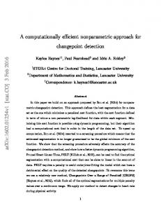
Percentage of label changes T2000 vs T3038 Percentage of label changes T1000 vs T3038 Test error T2000(induction) Test error T1000(induction) Test error T3038(transduction)

0.18

0.16

0.14

0.12

0.1

0.08

0.06

0.04

0.02

0

0

Induction vs. Transduction

When we add new points to the training set, two questions arise. First, do the f (xi ) change significantly? Second, how important is the difference between induction and transduction over a large amount of new points, in terms of classification performance? The experiments shown in fig. 1 have been made considering three training sets, T 1000, T 2000 and T 3038, containing respectively 1000, 2000 and 3038 samples (the results plotted are averaged on 10 runs with randomly selected T 1000 and T 2000). The first two curves show the percentage of unlabeled data in T 1000 and T 2000 whose label has changed compared to the labels obtained when training over T 3038 (the whole dataset). This validates our hypothesis that the f (xi ) do not change much when adding new training points. The next three curves show the classification error for the unlabeled data respectively on T 3038 \ T 2000, T 3038 \ T 1000 and T 3038 \ T 1000, for the algorithm trained respectively on T 2000, T 1000 and T 3038. This allows us to see that the induction’s performance is close to that of transduction (the average relative increase in classification error compared to transduction is about 20% for T 1000 and 10% for T 2000). In addi-

200

300

400

500

600

700

800

900

1000

Figure 1: Percentage of unlabeled training data whose label has changed when test points were added to the training set, and classification error in induction and transduction. Horizontal axis: number of labeled data. tion, the difference is very small for large amounts of labeled data as well as for very small amounts. This can be explained in the first case by the fact that enough information is available in the labeled data to get close to optimal classification, and in the second case, that there are too few labeled data to ensure an efficient prediction, either transductive or inductive. 5.1.2

5.1.1

100

Varying The Test Set Size

The previous experiments have shown that when the test set is large in comparison with the training set, the induction formula will not be as efficient as transduction. It is thus interesting to see how evolves the difference between induction and transduction as the test set size varies in proportion with the training set size. In particular, for which size of the test set is that difference comparable to the sensitivity of the algorithm with respect to the choice of training set? To answer this question, we need a large enough dataset to be able to choose random training sets. The whole Letters dataset is thus used here, and the binary classification problem is to discriminate the letters ’A’ to ’M’ from the letters ’N’ to ’Z’. We take a fixed test set of size 1000. We repeat 10 times the experiments that consists in: (i) choosing a random base training set of 2000 samples (with 10% labeled), and (ii) computing the average error on test points in transduction by adding a fraction of them to this base training set and solving the linear system (eq. 2), repeating this so as to compute the error on all test points. The results are shown in fig. 2, when we vary the number of test points added to the training set. Adding 0 test points is slightly different, since it corresponds to

0.25

Table 1: Comparative Classification Error of the Laplacian Algorithm (Belkin & Niyogi, 2003), W holeSet in Transduction and W holeSet in Induction on the MNIST Database. On the horizontal axis is the number of labeled examples and we use two different sizes of training sets (1000 and 10000 examples).

Test error 0.24

0.23

0.22

0.21

0.2

0.19

0

0.05

0.1

0.15

0.2

0.25

0.3

0.35

0.4

0.45

0.5

Figure 2: Horizontal axis: number of test points added in proportion with the size of the training set. Vertical axis: test error (in transduction for a proportion > 0, and in induction for the proportion 0). the induction setting, that we plot here for comparison purpose. We see that adding a fraction of test examples corresponding to less than 5% of the training set does not yield a significant decrease in the test error compared to induction, given the intrinsic variability due to the choice of training set. It could be interesting to compare induction with the limit case where we add only 1 test point at step (ii). We did not do it because of the computational costs, but one would expect the difference with induction to be smaller than for the 5% fraction. 5.2

COMPARISON WITH EXISTING ALGORITHM

We compare our proposed algorithm (alg. 1) to the semi-supervised Laplacian algorithm from (Belkin & Niyogi, 2003), for which classification accuracy on the MNIST database of handwritten digits is available. Benchmarking our induction algorithm against the Laplacian algorithm is interesting because the latter does not fall into the general framework of section 2. In order to obtain the best performance, a few refinements are necessary. First, it is better to use a sparse weighting function, which allows to get rid of the noise introduced by far-away examples, and also makes computations faster. The simplest way to do this is to combine the original weighting function (the Gaussian kernel) with k-nearest-neighbors. We define a new weighting function Wk by Wk (xi , xj ) = W (xi , xj ) if xi is a k-nearest-neighbor of xj or vice-versa, and 0 otherwise. Second, Wk is normalized as in Spectral Clustering (Ng et al., 2002), i.e. W k (xi , xj ) = q P 1 n

Wk (xi , xj ) . P r6=j Wk (xr , xk ) r6=i Wk (xi , xr )

Labeled Total: 1000 Laplacian W holeSettrans W holeSetind Total: 10000 Laplacian W holeSettrans W holeSetind

50

100

500

29.3 25.4 26.3

19.6 17.3 18.8

11.5 9.5 11.3

25.5 25.1 25.1

10.7 11.3 11.3

6.2 5.3 5.7

1000

5000

5.7 5.2 5.1

4.2 3.5 4.2

Finally, the dataset is systematically preprocessed by a Principal Component Analysis on the training part (labeled and unlabeled), to further reduce noise in the data (we keep the first 45 principal components). Results are presented in table 1. Hyperparameters (number of nearest neighbors and kernel bandwidth) were optimized on a validation set of 20000 samples, while the experiments were done on the rest (40000 samples). The classification error is averaged over 100 runs, where the train (1000 or 10000 samples) and test sets (5000 samples) are randomly selected among those 40000 samples. Standard errors (not shown) are all under 2% of the error. The Laplacian algorithm was used in a transductive setting, while we separate the results for our algorithm into W holeSettrans (error on the training data) and W holeSetind (error on the test data, obtained thanks to the induction formula)5 . On average, both W holeSettrans and W holeSetind slightly outperform the Laplacian algorithm. 5.3

APPROXIMATION ALGORITHMS

The aim of this section is to compare the classification performance of various algorithms: • W holeSet, the original algorithm presented in sections 2 and 3, where we make use of all unlabeled training data (same as W holeSetind in the previous section), • RSubsubOnly , the algorithm that consists in speeding-up training by using only a random subset of the unlabeled training samples (the rest is completely discarded), • RSubRR and RSubnoRR , the approximation algorithms described in section 4, when the subset is selected randomly (the second algorithm discards the part CRR of the cost for faster training), 5

See section 5.3 for the origin of the name W holeSet.

Table 2: Comparative Computational Requirements (n = number of training data, m = subset size) W holeSet RSubsubOnly RSubRR SSubRR RSubnoRR SSubnoRR

Time O(n3 ) O(m3 )

Memory O(n2 ) O(m2 )

O(m(n − m)2 )

O(m(n − m))

O(m2 (n − m))

O(m2 )

• SSubRR and SSubnoRR , which are similar to those above, except that the subset is now selected as in algorithm 3. Table 2 summarizes time and memory requirements for these algorithms: in particular, the approximation method described in section 4, when we discard the part CRR of the cost (RSubnoRR and SSubnoRR ), improves the computation time and memory usage by a factor approximately (n/m)2 . The classification performance of these algorithms was compared on three multi-class problems: LETTERS is the “Letter Image Recognition” dataset from the UCI MLR. (26 classes, dimension 16), MNIST contains the first 20000 samples of the MNIST database of handwritten digits (10 classes, dimension 784), and COVTYPE contains the first 20000 samples of the normalized6 “Forest CoverType” dataset from the UCI MLR. (7 classes, dimension 54). We repeat 50 times the experiment that consists in choosing randomly 10000 samples as training data and the rest as the test set, and computing the test error (using the induction formula) for the different algorithms. The average classification error on the test set (with standard error) is presented in table 3 for W holeSet, RSubsubOnly , RSubnoRR and SSubnoRR . For each dataset, results for a labeled fraction of 1%, 5% and 10% of the training data are presented. In algorithms using only a subset of the unlabeled data (i.e. all but W holeSet), the subset contains only 10% of the unlabeled set. Hyperparameters have been roughly estimated and remain fixed on each dataset. In particular, λ (in eq. 1) is set to 100 for all datasets, and the bandwidth of the Gaussian kernel used is set to 1 for LETTERS, 1.4 for MNIST and 1.5 for COVTYPE. The approximation algorithms using the part CRR of the cost (RSubRR and SSubRR ) are not shown in the results, because it turns out that using CRR does not necessarily improve the classification accuracy, as argued in section 4. Additionally, discarding CRR makes training significantly faster. Compared to W holeSet, typical training times with these specific settings show that RSubsubOnly is about 150 times faster, RSubnoRR 6

Scaled so that each feature has standard deviation 1.

Table 3: Comparative Classification Error (Induction) of W holeSet, RSubsubOnly , RSubnoRR and SSubnoRR , for Various Fractions of Labeled Data. % labeled

1% W holeSet RSubsubOnly RSubnoRR SSubnoRR 5% W holeSet RSubsubOnly RSubnoRR SSubnoRR 10% W holeSet RSubsubOnly RSubnoRR SSubnoRR

LETTERS

MNIST

COVTYPE

56.0 ± 0.4 59.8 ± 0.3 57.4 ± 0.4 55.8 ± 0.3

35.8 ± 1.0 29.6 ± 0.4 27.7 ± 0.6 24.4 ± 0.3

47.3 ± 1.1 44.8 ± 0.4 75.7 ± 2.5 45.0 ± 0.4

27.1 ± 0.4 32.1 ± 0.2 29.1 ± 0.2 28.5 ± 0.2

12.8 ± 0.2 14.9 ± 0.1 12.6 ± 0.1 12.3 ± 0.1

37.1 ± 0.2 35.4 ± 0.2 70.6 ± 3.2 35.8 ± 0.2

18.8 ± 0.3 22.5 ± 0.1 20.3 ± 0.1 19.8 ± 0.1

9.5 ± 0.1 11.4 ± 0.1 9.7 ± 0.1 9.5 ± 0.1

34.7 ± 0.1 32.4 ± 0.1 64.7 ± 3.6 33.4 ± 0.1

about 15 times, and SSubnoRR about 10 times. Note however that these factors increase very fast with the size of the dataset (10000 samples is still “small”). The first observation that can be made from table 3 is that SSubnoRR consistently outperforms (or does about the same as) RSubnoRR , which validates our subset selection step (alg. 3). However, rather surprisingly, RSubsubOnly can yield better performance than W holeSet (on MNIST for 1% of labeled data, and systematically on COVTYPE): adding more unlabeled data actually harms the classification accuracy. There may be various reasons to this, the first one being that hyperparameters should be optimized separatly for each algorithm to get their best performance. In addition, for high-dimensional data without obvious clusters or low-dimensional representation, it is known that the inter-points distances tend to be all the same and meaningless (see e.g. (Beyer et al., 1999)). Thus, using a Gaussian kernel will force us to consider rather large neighborhoods, which prevents a sensible propagation of labels through the data during training. Nevertheless, a constatation that arises from those results is that SSubnoRR never “breaks down”, being always either the best or close to the best. It is able to take advantage of all the unlabeled data, while focussing the computations on a well chosen subset. The importance of the subset selection is made clear with COVTYPE, where choosing a random subset can be catastrophic: this is probably because the approximation made in eq. 8 is very poor for some of the points which are not in the subset, due to the low structure in the data. Note that the goal here is not to obtain the best performance, but to compare the effectiveness of those algo-

rithms under the same experimental settings. Indeed, further refinements of the weighting function (see section 5.2) can greatly improve classification accuracy. Additional experiments were performed to asses the superiority of our subset selection algorithm over random selection. In the following, unless specified otherwise, datasets come from the UCI MLR, and were preprocessed with standard normalization. The kernel bandwidth was approximately chosen to optimize the performance of RSubnoRR , and λ was arbitrarily set to 100. The experiments consist in taking as training set 67% of the available data, 10% of which are labeled, and using the subset approximation methods RSubnoRR and SSubnoRR with a subset of size 10% of the available unlabeled training data. The classification error is then computed on the rest of the data (test set), and averaged over 50 runs. On average, on the 8 datasets tested, SSubnoRR always gives better performance. The improvement was not found to be statistically significative for the following datasets: Mushroom (8124 examples × 21 variables), Statlog Landsat Satellite (6435 × 36) and Nursery (12960 × 8). SSubnoRR performs significantly better than RSubnoRR (with a relative decrease in classification error from 4.5 to 12%) on: Image (2310 × 19), Isolet (7797 × 617), PenDigits (10992 × 16), SpamBase (4601×57) and the USPS dataset (9298×256, not from UCI). Overall, our experiments show that random selection can sometimes be efficient enough (especially with large low-dimensional datasets), but smart subset selection is to be preferred, since it (almost always) gives better and more stable results.

6

CONCLUSION

The first contribution of this paper is an extension of previously proposed non-parametric (graph-based) semi-supervised learning algorithms, that allows one to efficiently perform function induction (i.e. cheaply compute a prediction for a new example, in time O(n) instead of O(n3 )). The extension is justified by the minimization of the same smoothness criterion used to obtain the original algorithms in the first place. The second contribution is the use of this induction formula to define new optimization algorithms speeding up the training phase. Those new algorithms are based on using of a small subset of the unlabeled data, while still keeping information from the rest of the available samples. This subset can be heuristically chosen to improve classification performance over random selection. Such algorithms yield important reductions in computational and memory complexity and, combined with the induction formula, they give predictions close to the (expensive) transductive predictions.

References Belkin, M., Matveeva, I., & Niyogi, P. (2004). Regularization and semi-supervised learning on large graphs. COLT’2004. Springer. Belkin, M., & Niyogi, P. (2003). Using manifold structure for partially labeled classification. Advances in Neural Information Processing Systems 15. Cambridge, MA: MIT Press. Beyer, K. S., Goldstein, J., Ramakrishnan, R., & Shaft, U. (1999). When is “nearest neighbor” meaningful? Proceeding of the 7th International Conference on Database Theory (pp. 217–235). Springer-Verlag. Chapelle, O., Weston, J., & Scholkopf, B. (2003). Cluster kernels for semi-supervised learning. Advances in Neural Information Processing Systems 15. Cambridge, MA: MIT Press. Kemp, C., Griffiths, T., Stromsten, S., & Tenembaum, J. (2004). Semi-supervised learning with trees. Advances in Neural Information Processing Systems 16. Cambridge, MA: MIT Press. Nadaraya, E. (1964). On estimating regression. Theory of Probability and its Applications, 9, 141–142. Ng, A. Y., Jordan, M. I., & Weiss, Y. (2002). On spectral clustering: analysis and an algorithm. Advances in Neural Information Processing Systems 14. Cambridge, MA: MIT Press. Seeger, M. (2001). Learning with labeled and unlabeled data (Technical Report). Edinburgh University. Szummer, M., & Jaakkola, T. (2002). Partially labeled classification with markov random walks. Advances in Neural Information Processing Systems 14. Cambridge, MA: MIT Press. Watson, G. (1964). Smooth regression analysis. Sankhya The Indian Journal of Statistics, 26, 359–372. Williams, C. K. I., & Seeger, M. (2001). Using the Nystr¨ om method to speed up kernel machines. Advances in Neural Information Processing Systems 13 (pp. 682–688). Cambridge, MA: MIT Press. Zhou, D., Bousquet, O., Navin Lal, T., Weston, J., & Sch¨ olkopf, B. (2004). Learning with local and global consistency. Advances in Neural Information Processing Systems 16. Cambridge, MA: MIT Press. Zhu, X., Ghahramani, Z., & Lafferty, J. (2003a). Semisupervised learning using gaussian fields and harmonic functions. ICML’2003. Zhu, X., Lafferty, J., & Ghahramani, Z. (2003b). Semisupervised learning: From gaussian fields to gaussian processes (Technical Report CMU-CS-03-175). CMU.