Special ITC Section
Efficient Sequential Test Generation Based on Logic Simulation Shuo Sheng
Michael S. Hsiao
Rutgers University
Virginia Tech
A simple and highly efficient logic-simulationbased test generator uses a genetic algorithm to achieve both high fault coverage and short test generation times. ALTHOUGH RESEARCH on automatic test-pattern generation (ATPG) has yielded effective solutions for combinational circuits, developing efficient methods for sequential circuits remains difficult. The difficulty results because state and time frame expansion has caused a virtual explosion of the relevant search space. The commonly used branch-and-bound technique1 is infeasible for large sequential circuits because of the exponentially growing numbers of backtracks. In recent years, researchers have focused on simulation-based techniques2-7 because of their scalability to large circuits. We divide this class of test generators into fault simulation based4,6,7 and logic simulation based.2,5 In the former, a test generator repeats fault simulation runs to gather information on targeted faults to guide the test generator’s search for test sequences. In the latter, logic simulation makes up the bulk of computation, with minimal calls to fault simulation. Logic-simulation-based test generators usually target a property of the fault-free circuit and try to derive a sequence that exercises this property to a large extent. In research by Saab and colleagues,2 the test generator tries to maximize
2
0740-7475/02/$17.00 © 2002 IEEE
the circuit activity (events in logic simulation), whereas in research by Pomeranz and Reddy5 the test generator aims to maximize the number of new states visited. Recently, researchers have combined fault-simulation and circuit properties6,7 in cases where static test-set compaction yields the embedded properties. For example, compaction can identify useful vectors that can be repeated to detect additional faults;6 moreover, spectral properties embedded in the circuit under test can be extracted to assist generation of test vectors.7 Generally, because logic simulation is significantly less complex than fault simulation, execution time can be far shorter. However, the fault coverage of logic-simulation-based test generators, such as Cris2 and Locstep,5 can be inferior for large circuits when compared with that of fault-simulation-based, state-of-the-art test generators such as Strategate,4 Proptest,6 and Spect.7 In this article, we present an efficient logicsimulation-based test generator that executes significantly more quickly than its fault-simulationbased counterparts. This test generator’s fault coverage compares favorably with that of the latest techniques for large sequential circuits.
Motivation and concept Hard faults generally require reaching hardto-reach states during testing. Therefore, Pomeranz and Reddy5 developed a test generator that aims to drive the fault-free circuit to as many new states as possible. However, because large sequential circuits have many states reachable by testing, the fault coverage can IEEE Design & Test of Computers
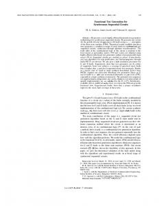
level off prematurely. This situation is often due to the indiscriminate addition of new states. Indiscriminate adding of new states is ineffective because some state variables belong to the data path and others belong to the control path, so maximizing the new states on the data path generally does not play as significant a role as maximizing those on the control path. This implies that we should not treat the entire state as a whole in optimization, because excessive noise from those unimportant states could misguide the test generator. Partitioning the state can help weed out the noise. Figure 1 shows how state partitioning can remove the noise and provide better guidance in the search space. Figure 1 shows a circuit with eight flip-flops. Let us partition global state S into partial states S1 and S2. We denote a distinct partial state as hexadecimal; for example, the number 5 represents partial state 0101 appearing on partition S1. We use the same notation for S2. For global state S, a couple (S1, S2) represents its value. For example, (5, A) represents global state 0101 1010. Assume the current test set has reached the following global states: (0, 0), (1, 1), (1, 2), (2, 3). The partial states visited on S1 and S2 are {0, 1, 2} and {0, 1, 2, 3}. Based on this state information, consider the following two scenarios. First, suppose two new candidate sequences drive the circuit from the current state to two new, different global states, (2, 1) and (3, 1). From the given starting state, we need select only one to append to the test set. If no distinction is made between these two global states, the test generator simply picks one randomly. However, state partitioning can differentiate the two states by pointing out that (3, 1) is more attractive because 3 brings a new state into partition S1, whereas both 2 and 1 have already been reached in the two separate partitions. Second, suppose the two different global states reached by the two candidate sequences are (3, 0) and (2, 4), and we need to pick only one to append to the test set. Both states are new global states; in addition, 3 is a new partial state on S1, and 4 is a new partial state on S2. By simply glancing at these two global states, it would be difficult to favor one over the other. However, imposing different weights on different state partitions lets us differentiate them. A September–October 2002
Global state S FF1 FF2 FF3 FF4 FF5 FF6 FF7 FF8
Partitioned states S1 and S2 FF1 FF2 FF3 FF4
Current state table
Example 1
Example 2
S1:
0
FF5 FF6 FF7 FF8
S2:
0
1
1
1
2
2
3
2
1
3
1
3
0
2
4
Figure 1. State partition examples. State partitioning can provide additional discrimination between states.
partition deemed to have greater influence on the circuit gets a greater weight. If the weight assigned to S1 surpasses that of S2, the algorithm chooses (3, 1). Our test generator combines logic simulation and state partition. Our proposed procedures include the following: ■ ■ ■
Divide the state into a set of partitions both statically and dynamically. Apply a genetic algorithm (GA) to maximize new states reached in each partition. Incorporate reset signal masking to avoid revisiting previously reached states, and thus expand the searched state space.
Initially, we do the partitioning statically according to the controllability of each flip-flop. As the fault coverage begins to become saturated, we invoke dynamic partitioning to regroup the flip-flops according to the structural analysis of the remaining undetected faults. Ideally, we would have a test sequence that can fully exercise the control path, so we want to explicitly distinguish between control and data paths. However, this is difficult, especially when
3
Special ITC Section
Table 1. Test generation (100,000 vectors) without and with reset signal masking. No reset signal masking Circuit
No. of
Execution
detected faults
time (s)
No. of
With reset signal masking No. of
vectors states
No. of
Execution
No. of
No. of
detected faults
time (s)
vectors
states
s1423
843
10.5
1,990
1,814
s5378
2,985
51.8
5,950
5,950
s35932
33,397
43.8
1,240
464
s38417
1,970
204.8
1,050
1,050
div16
1,691
20.2
5,990
5,492
1,669
20.6
6,000
5,655
951
54.2
1,070
112
6,600
1,000.1
11,010
10,807
b22 11,330 8,933.5 38,670 38,175 * No reset masking was applied, because all PIs have similar reset power.
20,081
8,159.2
33,380
33,760
b15
we are working with a gate-level circuit description. Therefore, we take an alternative approach that orients the partition to best suit our objective of achieving high fault coverage. We first partition the state into subgroups based on each flipflop’s controllability (FF controllability). We group flip-flops with similar ranges of controllability values together. Then we use a GA-based engine to search for a sequence that maximizes partitioned-state reachability.8 Another technique, reset signal masking, guides the search to avoid revisiting previously visited states for each partition. As test generation progresses, the test generator dynamically alters state partitioning using the circuit’s structural information that corresponds to the remaining undetected faults, to further improve fault coverage.
Reset signal masking We introduced the reset signal masking technique to help state traversal.9 Because our goal is to reach as many useful states as possible, our search must not frequently return the circuit to an old or reset state. Therefore, we want to mask those primary inputs (PIs) to a value that will prevent the circuit from being reset or partially reset. We use parallel simulation to identify the circuit’s reset or partial-reset PIs and perform the masking as part of the GA process. To demonstrate the effectiveness of reset signal masking, we implemented a test generation procedure that maximizes global state activity. In this procedure, we use the GA to optimize and pick, from a cluster of candidate sequences, the best sequence that maximizes
4
1,044
15.7
2,850
2,822
No reset masking applied* 35,100
25.0
568
568
No reset masking applied*
the number of global states visited. The sequence length is 10. We append the selected best sequence to the test set. The test generator performs this procedure repeatedly until a total of 100,000 vectors are generated. For global states, we consider all flip-flop values in deciding if a new state appears in a state table. This is in contrast to partial states, which result from state partitioning. We tested the test generation procedure both with and without reset signal masking.1 We ran both experiments on a Pentium 4, 1.8GHz machine with 512 Mbytes of RAM and the Linux operating system. As the results in Table 1 show, in circuits s1423, s35932, b15, and b22, reset masking greatly improved the fault coverage—for example, in s1423, reset signal masking helped detect 201 more faults than without signal masking. For b15 and b22, this difference increased to about 5,649 and 8,751. In s35932, the fault coverage reached in just 25 seconds was almost as high as reported by far more complex sequential test generators such as Strategate and Proptest, which require hours of computation. For circuits s5378 and s38417, no reset masking was applied because no biased reset PI was available.
State partitioning methods Although reset signal masking can yield excellent fault coverage results, the coverage we attained was still not as high as that obtained by state-of-the-art sequential test generators. By adding state partitioning to our test generation framework, we can detect still more IEEE Design & Test of Computers
faults, and our results match those achieved by other researchers for many circuits.4,6,7 Random partitioning As Figure 1 shows, we must address two problems to accomplish state partitioning: ■ ■
how to group flip-flops into different partitions, and how to assign weights to different partitions.
Table 2. Test generation (100,000 vectors) without and with random state partitioning. No partitioning Circuit
N −1
∑ {W
j
×U j
j =0
No. of
Execution
detected faults
time (s)
detected faults
time (s)
1,044
15.7
1,414
8,394.0
s5378
2,985
51.8
3,588
4,894.0
s35932
35,100
25.0
35,100
25.0
s38417
1,970
204.8
1,970
190.8
div16
1,669
20.6
1,808
3,005.0
b15
6,600
1,000.1
16,954
10,778.0
b22
20,081
8,159.2
23,437
20,481.0
}
where N is the total number of partitions (we set it to 5), and Wj is the weight assigned to partition Sj. Uj = 10 if the partial state on partition Sj is a new state in its partial table, Tj. Uj = 1/ns if the partial state on partition Sj is an old state for Tj, where ns is the number of times this partial state has been visited during logic simulation. This fitness function gives preference to both September–October 2002
Execution
s1423
We first attempt the simplest partitioning heuristic—random partitioning and random weights—to show how even simple partitioning can influence test generation results. In random partitioning, given N partitions, the state variables are randomly and evenly distributed into N groups, each group (except the last one) having the same number of flip-flops. We randomly assign integer weights from 1 to N to these N groups, denoted by partition Sj, j = 0, … , N – 1. During logic simulation, we store statistics of both global states and partition states into two separate tables: global state table Tglobal, which stores every distinct full state reached in logic simulation, and partitioned state tables T0, … , TN–1, which contain the projection of the full state onto each of the ith partitions. Therefore, each partition Sj manages a state table, Tj. After we determine the state partition and partition weights, we invoke the same test generation procedure as used earlier. But the fitness function in a GA is more complex because of the state partition. We compute it as the following formula: fitness =
Random partitioning
No. of
new and less-visited states appearing in strongly biased state partitions (with higher Wj values). We compute the fitness by simulating each candidate sequence in the GA population. Parallel logic simulation evaluates 32 candidate sequences simultaneously to reduce computational cost. No fault simulation is involved until the GA has selected the best candidate sequence to add to the test set. At that point, fault simulation drops the faults detected by this sequence. The sequence length is set to 10 for all simulations. Thus, the test set grows at a rate of 10 vectors for every GA optimization procedure. We ran the same test generation procedure for the partitioning method as we did with reset signal masking but with random-state-partitionbased fitness incorporated into the GA engine. Table 2 lists our results for two cases: without and with random-state partitioning. We applied reset signal masking in both cases. In this table, the results reported under the column “No partition” are identical to those shown in Table 1 under the column “With reset signal masking.” As Table 2 shows, random partitioning has significantly improved fault coverage for most circuits. For s1423, the number of detected faults reached 1,414, which is as high as results achieved with Strategate. For s5378, div16, b15, and b22, the improvement was also quite dramatic. The exceptions are s35932 and s38417. For the former, since the fault coverage achieved by reset signal masking was already very high, state partitioning yielded minimal benefit. For the latter, we believe that the s38417 circuit requires intelligent partitioning methods rather than random partitioning.
5
Special ITC Section
Table 3. Test generation (100,000 vectors) with FF-controllability-based partitioning.
Circuit
No state partitioning
Random partitioning
No. of
Execution
No. of
Execution
No. of
Execution
detected faults
time (s)
detected faults
time (s)
detected faults
time (s)
s1423
1,044
15.7
1,414
8,394.0
1,415
2,980.2
s5378
2,985
51.8
3,588
4,894.0
3,615
2,167.2
s35932
35,100
25.0
35,100
25.0
35,100
25.0
s38417
1,970
204.8
1,970
190.8
2,024
1,128.1
div16
1,669
20.6
1,808
3,005.0
1,855
3,061.0
b15
6,600
1,000.1
16,954
10,778.0
18,314
8,907.8
b22
20,081
8,159.2
28,437
20,481.0
30,493
27,924.0
FF-controllability-based partitioning In a given sequential circuit, some state variables are less controllable than others. Less activity typically occurs in these flip-flops. For the circuit to traverse more useful states, it is often desirable to stimulate more activity on these less-active flip-flops. Therefore, the first intelligent partitioning method we employ is based on FF controllability. We perform a logic simulation of N random vectors (typically, N is set from 500 to 1,000) and record the number of times each FFi is set to 0 and 1, denoted by Ni0 and Ni1. The 0 controllability of FFi is calculated as CC0i = Ni0/N, and the 1 controllability is CC1i = Ni1/N. We define the absolute value of the difference of the controllability values and call it FFbias: FFbias(i) = |CC0i – CC1i| If FFbias(i) is close to 0, then FFi is easily controlled as both 0 and 1. A large FFbias(i) indicates that a strong bias exists for this flip-flop. We do not further differentiate it as a bias-to-0 or 1, because we are most concerned with reducing this bias in state traversal. To partition the state, we group each FFi into a subgroup Sj, according to its bias value. Five bias value ranges are considered: {ai, ai+1}, where ai = {0.0, 0.2, 0.4, 0.6, 0.8, 1.0}. If the bias value of FFi falls into any of these five ranges—for example, {aj, aj+1}—then FFi is grouped into subgroup Sj. The number of flip-flops in each subgroup Sj is the size of the partition. We also assign a weight Wj for each Sj, just as subgroups with larger bias values are assigned larger weights.
6
FF-control partitioning
Table 3 shows how FF-controllability-based partitioning, with reset signal masking, can yield more improvements over no partitioning and random partitioning. The results for no partitioning and random partitioning are the same as those in Table 2. You can see from Table 3 that for circuit s1423, one more fault was detected than with random partitioning, and the time was reduced by about 75%. For s5378, 27 more faults were detected and the time was nearly halved. We observed the same phenomenon for div16, s38417, b15, and b22. Particularly for div16, the number of detected faults (1,855) already surpassed those detected by Strategate (1,614) and Proptest (1,652). Structure-based partitioning Although FF-controllability-based partitioning with GAs and reset signal masking has achieved far higher fault coverage than previous methods, it has not yet matched the results reported by other complex sequential test generators. The reason is that the fault coverage becomes saturated when the partition cannot provide further guidance for those hard faults. This is because the FF-controllability-based partitioning primarily targets the harder-to-control flip-flops. For the remaining hard faults, we need to further refine the search space; we need fault-related information to adjust the partitioning when the fault coverage begins to level off. This leads to dynamic partitioning—a more intelligent and adaptive partitioning method— using the undetected faults’ structural information. IEEE Design & Test of Computers
In Pomeranz and Reddy’s work,10 a dynamically selected subcircuit (instead of the complete circuit) reduces the test generation cost. Chickermane and Patel, on the other hand, proposed a fault-oriented method for choosing flipflops for partial scan.11 Both methods attempt to associate the circuit’s structural information with the fault site. We followed similar steps to locate those flip-flops that have more influence on excitation and propagation of the remaining faults and group them together. We use the algorithm in Figure 2 to score each flip-flop according to its structural location related to the target faults: In the above algorithm, the influencing cone is the fan-in cone for signals on the fault’s propagation path. Typically, N and M are set to 100 and 5. Figure 3 shows an example. The fault site is marked X in the figure. According to the definition, FF1 and FF2 are in the fault’s fan-in cone; they will influence the fault’s excitation. FF3 and FF4 are in the fault’s influencing cone, so they control the fault’s propagation. Wexcite and Wprop are the weights that the algorithm gives to the flip-flop, depending on where it is located. These two values are set to either 5 or 10. If the fault has been activated, we weight propagation more than excitation; otherwise, we give more weight to excitation.
Experimental results Here we report the experiments we performed with our proposed logic-simulationbased test generator and the results we achieved on several benchmark and industry circuits. Test generation We implemented the dynamic partitioning (structure-based) algorithm and integrated it into our test generation procedure. We executed the program on several ISCAS 89 (International Symposium on Circuits and Systems) and ITC 99 (International Test Conference) benchmark circuits and two industry circuits, GPIO (GeneralPurpose Input-Output bus controller) and Paulin.12 Because state partitioning is the core of the algorithm, this test generator targets large sequential circuits having more than 50 flip-flops. However, we also report results for two circuits September–October 2002
//Step 1: Select target fault set Choose target fault set F from activated but undetected fault set, or previously excited but undetected fault set, or random sampling of undetected fault set. //Step 2: Conduct structural analysis for each fault fi in target fault set F for each FFj in the state if FFj is in the fan-in cone of fi then FF_score(j) + = Wexcite; if FFj is in the influencing cone of fi FF_score(j) + = Wprop; //Step 3: Sort flip flops Sort flip-flops according to their FF_score value //Step 4: Partition flip-flips Pick first N flip-flops with biggest FF_score, and divide them equally into M partitions.
Figure 2. Algorithm to score flip-flops according to structural location.
FF1 FF2
FF3
Gate 1
X
Gate 2
Gate 3
Primary output
FF4
Figure 3. Example of fault-oriented structural analysis.
with fewer than 50 flip-flops—s400 and s641—to illustrate the effectiveness on smaller circuits. In Table 4 (next page), we report the test generation results for these circuits by the following test generators: ■
■ ■
■
Locstep,5 a logic-simulation-based test generator that targets maximizing global states visited (no state partitioning); Hitec,1 a deterministic test generator; Strategate,4 a GA- and fault-simulation-based test generator (using a Hewlett-Packard 9000 J200 machine with 256 Mbytes of memory); and Proptest,6 a compaction-, fault-simulationbased test generator (using a Pentium II 400MHz workstation).
7
Special ITC Section
Table 4. Test generation results from existing test generators.* Locstep5 No. of
Circuit
Strategate4
No. of
detected
No. of
Execution
detected
faults
vectors
faults
vectors
time (s)
faults
s641 1,274
9,616
Proptest6
No. of
Detected
s400
s1423
Hitec1,12 No. of
382
No. of No. of Execution vectors
time (s)
382
4,309
2,424
404
216
404
166
776
177
1,414
3,943
4,572
detected No. of Execution faults
vectors time (s)
382
617
92
404
182
30
1,416
1,387
277
s5378
3,059
7,545
3,238
941
3,639
11,571
136,080
3,643
706
898
s35932
34,812
2,408
34,902
240
35,100
257
39,240
35,101
255
676
2,006
30,802
1,835,861
1,665
189
1,814
3,476
29,160
1,852
243
b15
17,921
83,465
1,515,498
18,257
58,244
b22
30,788
22,059
196,513
30,678
50,723
s38417 div16
GPIO
2,865
1,396
57
2,833
5,292
11,078
Paulin
67,909
752
147,002
69,150
4,499
101,071
* Blank entries indicate that the data was not available; no execution times were available for Lockstep.
Table 5 lists our experimental results. We applied reset signal masking in all cases, which generated 100,000 vectors. In the rightmost column under “Dynamic partition,” we show the test generation results with dynamic state partitioning applied. In the three other cases, we list results obtained with no partitioning, random partitioning, and FF-controllability-based static partitioning. For each circuit, we list the number of detected faults and test generation time from each method. Comparing our results from Table 5 to those in Table 4 shows that our dynamic-partition-based test generator has achieved fault coverage comparable to Strategate, as well as to Proptest on hard-to-test circuits, generally with a shorter execution time. For example, for circuit s1423, Strategate detected 1,414 faults in 4,572 seconds, Proptest detected 1,416 faults in 277 seconds, and ours detected 1,415 in 147 seconds. Results were most dramatic with circuit b15. For b15, Strategate detected 17,921 faults with 83,465 vectors in 1,515,498 seconds, and Proptest detected 18,257 faults in 58,244 seconds. Our dynamic partitioning technique detected the most faults—18,276—in only 4,555 seconds. For circuit s35932, the execution time was far shorter than all the others. For div16 and s38417, our approach also achieved the highest fault coverage. Likewise, the performance was also far bet-
8
ter than Hitec’s and Locstep’s for all circuits. For the two industrial circuits, GPIO and Paulin, our methods showed significant performance improvement in execution time over Hitec and Strategate, although the fault coverage yielded was about the same in GPIO and slightly higher in Paulin. The results were similar for the two smaller circuits, s400 and s641. Table 5 also shows that a dynamic-partitionbased approach can speed up the test generation time against the static-partition-based approach. For example, for s1423, although both approaches detected 1,415 faults, the dynamic approach reduced the time from 2,890 seconds in the FF-controllability-based approach to 147 seconds. The GPIO circuit is a typical example, showing how dynamic partitioning outperforms the static-partitioning and no-partitioning methods. The number of detected faults climbed to 2,843 with dynamic partitioning, whereas the no-partitioning and random-partitioning methods remained below 1,000, and FF-controllabilitybased partitioning remained below 2,000. Circuit b15 is a different case, in which the dynamic-partitioning approach performed worse than static partitioning. The reason was that our dynamic partitioning algorithm is a heuristic and might not always provide the correct searching direction. IEEE Design & Test of Computers
Table 5. Our test generation results using the state partition technique. No partitioning No. of Circuit s400 s641 s1423
Random partitioning No. of
FF-controlled partitioning
Dynamic partitioning
No. of
No. of
detected
Execution
detected
Execution
detected
Execution
detected
Execution
faults
time (s)
faults
time (s)
faults
time (s)
faults
time (s)
382
8.75
382
8.30
380
10.70
382
9.00
404
6.60
404
13.80
404
6.68
404
6.83
1,044
15.70
1,414
8,394.00
1,415
2,980.20
1,415
147.00
s5378
2,985
51.80
3,588
4,894.00
3,615
2,167.20
3,636
212.00
s35932
35,100
25.00
35,100
25.00
35,100
25.00
35,100
24.00
s38417
1,970
204.80
1,970
190.80
2,024
1,128.10
2,228
2,149.00
div16
1,669
20.60
1,808
3,005.00
1,855
3,061.00
1,873
771.00
b15
6,600
1,000.10
16,954
10,778.00
18,314
8,907.80
18,276
4,555.00
b22
20,081
8,159.20
28,437
20,481.00
30,493
27,924.00
30,684
16,914.00
GPIO
635
5,681.00
405
2.92
1,858
999.70
2,843
174.30
Paulin
69,020
385.00
68,967
362.00
69,173
253.00
69,173
192.30
For large circuits like div16, b15, and b22, our test generation times were longer because of the fault simulation of the 100,000 generated vectors. In fact, 90% of the test generation was spent on fault-simulating the test set. Test-set compaction The number of test sets generated by our approach in Table 5 was high (an upper limit of 100,000 vectors were generated for each circuit). Generally, this class of test generators yields longer test sets than deterministic or compaction-based methods. However, with a postcompaction step, we can reduce the test sets significantly. We applied a static test-set compaction procedure to the test sets generated by our method; Table 6 shows the results. The “Original test length” column reports the actual test-set length corresponding to the fault coverage achieved in Table 5. The “Compacted test length” column reports the test-set length after compaction. For instance, for s5378, the original test set of 12,144 vectors was compacted to only 1,123 vectors, to achieve the same fault coverage. Likewise, in circuit s35932, the initial test-set length by our technique was 568. After compaction, only 208 vectors are needed to achieve the same coverage. This sequence of 208 vectors is shorter than the test sets obtained by either Strategate or Proptest. The results show that the disadvantage of an initially longer test September–October 2002
Table 6. Test compaction results. Circuit
Original test length
Compacted test length
(no. of vectors)
(no. of vectors)
s1423
16,110
1,334
s5378
12,144
1,123
s35932
568
208
s38417
8,100
5,415
div16
37,951
10,278
b15
79,060
17,251
b22
99,080
31,065
GPIO
15,999
8,142
Paulin
2,230
404
sequence in our technique can easily be remedied by efficient compaction procedures.
WE HAVE PRESENTED an efficient, yet simple,
sequential test generator that uses logic simulation. Through state partitioning, we can further discriminate candidate states and thus effectively guide the search engine to detect hard faults. Future work in this area includes developing more delicate dynamic algorithms for state partitioning. Various partial-scan algorithms in DFT can be migrated to this domain. Such algorithms are generally considered FFprioritizing schemes, which are naturally suitable for partitioning. ■
9
Special ITC Section
Acknowledgments
Based Test Generation for Combinational Circuits
This research was supported in part by the National Science Foundation under grant CCR0196470, a grant from the New Jersey Commission on Science and Technology, and a grant from Fujitsu Labs of America.
Using Dynamically Selected Subcircuits,” Proc. Int’l Conf. Computer Design (ICCD 99), IEEE CS Press, Los Alamitos, Calif., 1999, pp. 412-417. 11. V. Chickermane and J.H. Patel, “A Fault Oriented Partial Scan Design Approach,” Proc. Int’l. Conf. Computer-Aided Design (ICCAD 91), IEEE CS
References 1. T.M. Niermann and J.H. Patel, “HITEC: A Test
Press, Los Alamitos, Calif., 1991, pp. 400-403. 12. I. Ghosh and M. Fujita, “Automatic Test Pattern
Generation Package for Sequential Circuits,”
Generation for Functional Register-Transfer Level
Proc. European Design Automation Conf. (EURO-
Circuits Using Assignment Decision Diagrams,”
DAC 91), IEEE CS Press, Los Alamitos, Calif.,
IEEE Trans. Computer-Aided Design of Integrated
1991, pp. 214-218.
Circuits and Systems, vol. 20, no. 3, Mar. 2001.
2. D.G. Saab, Y.G. Saab, and J.A. Abraham, “CRIS: A Test Cultivation Program for Sequential VLSI Circuits,” Proc. Int’l Conf. Computer-Aided Design (ICCAD 92), IEEE CS Press, Los Alamitos, Calif., 1992, pp. 216-219. 3. E.M. Rudnick et al., “Application of Simple Genetic Algorithms to Sequential Circuit Test Generation,” Proc. European Design and Test Conf. (ED&TC 94), IEEE CS Press, Los Alamitos, Calif., 1994, pp. 40-45. 4. M.S. Hsiao, E.M. Rudnick, and J.H. Patel, “Sequential Circuit Test Generation Using Dynamic State Traversal,” Proc. European Design and
Shuo Sheng is a PhD student in the Department of Electrical and Computer Engineering at Rutgers University, Piscataway, New Jersey. His research interests include ATPG and formal verification. Sheng has a BS in automatic control from Huazhong University of Science & Technology, Wuhan, China, and an MS in electrical engineering from Tsinghua University, Beijing. He is a student member of the IEEE.
Test Conf. (ED&TC 96), IEEE CS Press, Los Alamitos, Calif., 1996, pp. 22-28. 5. I. Pomeranz and S.M. Reddy, “LOCSTEP: A Logic-Simulation-Based Test Generation Procedure,” IEEE Trans. CAD of Integrated Circuits and Systems, vol. 16, no. 5, May 1997, pp. 544-554. 6. R. Guo, I. Pomeranz, and S.M. Reddy, “A Fault Simulation Based Test Pattern Generator for Synchronous Sequential Circuits,” Proc. VLSI Test Symp. (VTS 99), IEEE CS Press, Los Alamitos, Calif., 1999, pp. 260-267. 7. A. Giani et al., “Efficient Spectral Techniques for Sequential ATPG,” Proc. IEEE Design Automation and Test in Europe Conf. (DATE 01), IEEE CS
Michael S. Hsiao is an associate professor in the Bradley Department of Electrical and Computer Engineering at Virginia Tech, Blacksburg, Virginia. His research interests include VLSI and SoC testing, design verification, diagnosis, and low-power design. Hsiao has a BS in computer engineering and an MS and PhD in electrical engineering, all from the University of Illinois at Urbana-Champaign. He is a member of the IEEE and the ACM.
Press, Los Alamitos, Calif., 2001, pp. 204-208. 8. D.E. Goldberg, Genetic Algorithms in Search, Optimization, and Machine Learning, AddisonWesley, Reading, Mass., 1989. 9. S. Sheng, K. Takayama, and M.S. Hsiao, “Effec-
Direct questions and comments about this article to Shuo Sheng, Dept. of Electrical and Computer Engineering, Rutgers University, Piscataway, NJ 08854;
[email protected].
tive Safety Property Checking Using SimulationBased Sequential ATPG”, Proc. Design
For further information on this or any other comput-
Automation Conf. (DAC 02), ACM Press, New
ing topic, visit our Digital Library at http://comput-
York, 2002, pp. 813-818.
er.org/publications/dlib.
10. I. Pomeranz and S.M. Reddy, “Fault Simulation
10
IEEE Design & Test of Computers