Efficient Structured Parsing of Façades Using Dynamic Programming

Efficient Structured Parsing of Fac¸ades Using Dynamic Programming Andrea Cohen1 , Alexander G. Schwing2∗, Marc Pollefeys1 1

ETH Z¨urich, Switzerland

2

University of Toronto, Canada

{acohen,pomarc}@inf.ethz.ch

[email protected]

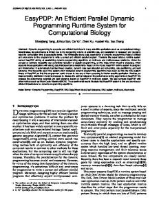
Abstract 50 100

y

1

We propose a sequential optimization technique for segmenting a rectified image of a fac¸ade into semantic categories. Our method retrieves a parsing which respects common architectural constraints and also returns a certificate for global optimality. Contrasting the suggested method, the considered fac¸ade labeling problem is typically tackled as a classification task or as grammar parsing. Both approaches are not capable of fully exploiting the regularity of the problem. Therefore, our technique very significantly improves the accuracy compared to the state-of-the-art while being an order of magnitude faster. In addition, in 85% of the test images we obtain a certificate for optimality.

200 250 300 50

100

150 y

200

250

300

2

(a)

(b) Error: 6.7%

(c)

Figure 1. The fac¸ade in (a) and our obtained parsing overlaying the image in (b) while the sparse green pattern in (c) indicates the efficiency of our proposed approach.

fac¸ades are well-organized, e.g., into floors that are in turn divided into repetitive elements. Naturally, those structural concepts impose constraints on the semantic labeling of a monocular image that should be beneficially exploited. Considering the monocular image understanding literature, many approaches possess no global guarantees. The strong interplay between designing an appropriate cost function and a corresponding algorithm for its rigorous optimization has, according to our opinion, been forgotten in the past few years where many tasks are formulated as labeling problems. Some exceptions are the room layout estimation of [26] and finding the globally optimal bounding box given classifier scores [16, 2]. We argue that construction of applications on top of scene interpretations, e.g., by predicting affordances [8] or by investigating the interactions between humans and objects [6], requires fast yet well performing algorithms preferably possessing guarantees or returning optimality certificates, i.e., indications of when the obtained result is guaranteed to be optimal. It seems ambitious to parse a fac¸ade like the one illustrated in Fig. 1(a) into semantic regions (Fig. 1(b)) to obtain a globally optimal labeling or at least certificates for global optimality. Nevertheless, we present an optimization problem for which we can construct optimality certificates while being more efficient if not interested in their computation. We first present an appropriate optimization problem and afterwards discuss usage of a dynamic programming algorithm with extensions for improved expected case efficiency. The latter amendment guarantees a sparse number of calls to the dynamic programming algorithm as

1. Introduction Monocular scene understanding is a long-standing goal in computer vision. Just by looking at a single image, humans are able to infer information like depth and, more importantly, relational structures, i.e., dependencies between different and possibly partly occluded objects. Humans are even able to come up with a short image sequence preceding and succeeding a presented scene. However, none of our algorithms are anywhere close to realistically achieving this ability when given a single input image. Nevertheless, there is an increasing amount of applications that successfully leverage monocular cues. Some notable examples are prediction of room layouts [10, 17, 35, 25] when considering indoor scenes, as well as automatic photo-popup [11], Make3D [22] and fac¸ade parsing approaches [32, 31, 18] when considering the outdoor setting. Common to many of those approaches, and in particular the fac¸ade parsing methods, is the initial formulation as a pixel-wise labeling task using standard classifiers with optional extensions to more complex structured prediction methods. However, those approaches often operate on individual pixels or super-pixels. While a super-pixel segmentation respects the edge-structure observed within an image to some extent, a pixel-wise classification is significantly more flexible. Nonetheless, most of our man-made structures and ∗ This

150

work was done while at ETH Z¨urich

1

illustrated in Fig. 1(c) where green pixels denote actual calls while otherwise, evaluation of the algorithm would have been required for every element of the entire uppertriangular matrix. All in all, our proposed algorithm requires individual executions of a dynamic program to find a labeling. Global optimality certificates are obtained if the individual algorithms remain independent. We illustrate the efficacy on two standard datasets being the “Ecole Centrale Paris Facades Database” and the “Zurich Building Dataset”, as well as the “eTRIMS database” with our quantitative evaluation on the first set indicating a 5.8% improvement compared to current state-of-the-art while reducing computational cost by an order of magnitude.

2. Related Work Parsing the rectified image of a fac¸ade has long been a prominent example for monocular scene understanding with early approaches dating back to the seminal work of Stiny [29]. Meanwhile, a multiplicity of methods on extraction and parsing of fac¸ades were proposed. While extraction is the focus in [38, 21], modeling was considered by the authors of [37, 19] and parsing in particular was also recently discussed by [32, 31, 18] and references therein. [32, 31] formulate the parsing problem by sampling from a grammar restricting the space of possible parses. Sampling accepts a new explanation once it scores higher than the best previously found parsing. However, nonprobabilistic optimality certificates for efficiently finding the global optimum are not known since the strategy for searching the state space is still largely random. Another approach based on Recursive Neural Networks was proposed in [18] and shown to outperform previously existing methods. The authors present a three-layer approach with the middle layer being a pairwise multi-label Markov Random Field (MRF) solved via a graph-cut algorithm. A graphcut formulation is only optimal for binary MRFs with submodular pairwise energies and hence the solution for the multi-label MRF in [18] does not even possess optimality certificates. More importantly though, the resulting labeling respects the structure introduced by the super-pixels. Although those super-pixels follow the edge structure to some extent, no guarantee exists for finding a visually pleasing explanation that follows common architectural patterns. Those were introduced within an independent third layer and shown to slightly decrease labeling accuracy while occasionally producing visually more pleasing results. Hence, currently existing approaches exhibit no optimality certificates upon having found the parsing of a fac¸ade. This is, however, true for many tasks considered within computer vision with a few exceptions. Importantly, there is a wide range of applications based on branch-and-bound inference with examples ranging from object localization [16] via landmark detection for model fitting to images [1], to camera parameter detection [9] [20]. Other examples are

based on maximum sum sub-array and maximum sum submatrix [5] algorithms like [2]. Tasks that involve inference over tree-structured graphs or graphs with low tree-width are solved via dynamic-programming like message passing techniques which are suitable for 2D scene labeling with a specific structure as in [7]. Dynamic programming can also be used for optimal 1D labeling for stereo [23] and more general models in case a binary labeling is obtained. Graph cut is the method of choice for binary MRFs with sub-modular pairwise energies, which is applied to a number of (low-level) vision tasks like binary image denoising and binary labeling, as described in [13]. Similar tasks can be achieved via linear programming relaxations [36]. Optimality certificates and efficient algorithms are – according to our opinion – important for computer vision since they shift the focus from the design of a large system with many parameters to the design of features that represent valuable information for a specific application. Subsequently we are interested in providing an efficient method for the task of parsing a fac¸ade which can provide optimality certificates. Our approach follows the dynamic programming paradigm and is detailed as follows.

3. Approach We are interested in parsing every pixel of an image illustrating a rectified fac¸ade into semantic categories subsumed within the following label set L = {sky, chimney, roof, window, balcony, wall, door, shop}. While this problem is fairly complex in general, typical fac¸ades exhibit a specific structure which greatly simplifies the parsing procedure. We therefore argue subsequently that exploiting these architectural constraints improves the performance of a pixel-wise labeling task w.r.t. both computational complexity as well as accuracy. Let z ∈ Z denote a parsing of a fac¸ade and assume that Z denotes the exponentially sized set of all possible pixelwise image labelings. Clearly many of those parsings, like randomly choosing a semantic label for every pixel, are not at all reasonable when considering the regularity of manmade structures. Due to the common rectangular structure of fac¸ades, we rather let the set Z be described by a product space with every member denoting a rectangular box. Importantly, the size of this set, i.e., the number of boxes involved, is not specified a-priori but rather determined when explaining the observed image which is assumed to be of quadratic dimension N ×N for notational convenience only. As usual, we measure the quality of the structured parsing z ∈ Z using a score function X S(z) = si (zi ) (1) i∈{1,...,N }2

summing for every pixel i within the image a score s that depends on the pixel label zi ∈ L induced by the parsing z. The score si of pixel i for label zi is the normalized log-

likelihood output of a classifier, i.e., si (zi ) = log pi (zi ) − P log l∈L pi (l) where pi is the multinomial probability distribution of pixel i over the label space L. Given the classifier scores and without constraints, the global maximum of this log-likelihood is easily found by assigning a pixelsized box with label arg maxzi si (zi ) to every pixel i. Such a labeling is not very accurate as it ignores constraints on fac¸ade layouts. We are, hence, interested in an approach enforcing more structure by maximizing the log-likelihood ratio while respecting common architectural constraints subsumed within the set C. This set consists of the following constraints: all fac¸ade elements (door, windows, roof, balconies) are represented by a rectangular box, balconies are required to be located below windows and to have at least the same width, all pairs of window/balcony lying on the same floor have the same height, the shops are located on the bottom, chimneys originate from the top of the roof, the fac¸ade and the roof cover the entire width of the image. Note that we operate with hard constraints rather than the typical soft constraints included into MRF formulations via Potts-type potentials. This strong structure allows to explain up to 98% of the ground-truth labelings used in our experiments, making them more accurate in some cases. We further emphasize and visualize in the experimental section that the set C is general enough to represent typical fac¸ades. Overview: We start by outlining our approach for parsing a fac¸ade given a rectified image. In particular, we will find a maximizer of the score given in Eq. (1) subject to the aforementioned architectural constraints C. The procedure is visually outlined in Fig. 2. We assume all the pixels to be initially assigned the label wall (see Fig. 2(a)) and begin by finding window-balcony rows throughout the image. The scores used during this stage are those of windows minus wall and balcony minus wall. For the detection of a single row of window-balcony, we use a chain-like dynamic program along the width of the image, i.e., along the x-coordinate. We only allow certain transitions between the variables and provide details when discussing Alg 2. To successively explain multiple window-balcony rows we pursue a recursive approach which investigates image parts above and below previously labeled areas. The results of this first step are illustrated in Fig. 2(b). In a second step we use a variant of our dynamic program to detect a combination of door and shop, such that the shop starts at the bottom of the image, and the door lies within the vertical boundaries of the shop. The top limit of the shop is found by exhaustive search of the best door-shop combination. A cost is payed for replacing any previous labelings with shop and door. This is illustrated in Fig. 2(c). In a third and last step, we jointly optimize for the labels roof, sky and chimney. To this end, we optimize exhaustively for two y-coordinates restricting the interior of the roof where we replace previously assigned labels with roof and at the same time optimize for a row of window/balcony inside these boundaries by using window/balcony vs. roof

(a) Step 0

(b) Step 1

(c) Step 2

(d) Step 3

Figure 2. Output for each step of our fac¸ade parsing procedure.

scores. Similarly, all pixels above the y-coordinate denoting the separation between roof and sky are relabeled from the previous labeling to sky while finding chimneys is done similarly to the search for windows (later described as DP1). However, we allow chimneys to have different heights while starting at the same y-coordinate offset. This final step retrieves a maximizer of Eq. (1) subject to constraints C as illustrated in Fig. 2(d). Finding a row of elements: Consider a task where we are interested in finding an intermittent rectangular pattern with heights being given by y1 and y2 . Requiring all elements to be rectangular, and assuming that all elements share the same vertical limits, we are hence interested in finding the highest scoring row of rectangular boxes {zk } with zk = (xk,1 , xk,2 , y1 , y2 ) ∈ {1, . . . , N }4 that share the same (y1 , y2 ) coordinates. Besides a row of windows, this can describe a row of balconies, an interrupted line of shops, etc. The score of each box SWindow (z) is given (in the case of a row of windows) by adding the log-likelihood output s of all interior pixels being window while subtracting the score of being wall. Having assumed all the pixels to be wall at first is the reason for the subtraction since we replace a wall label with a window label. We propose a dynamic programming approach that, given a pair of coordinates (y1 , y2 ), finds the maximum scoring set of boxes zk = (xk,1 , xk,2 , y1 , y2 ) in O(N ). We will refer to this algorithm as DP1. DP1 is a version of Viterbi’s algorithm [34] with 2 states representing the presence or the absence of the element of interest, e.g., window. It was also inspired by Kadane’s algorithm [4] which can find the best scoring box. For each column of pixels in a row bounded by (y1 , y2 ), DP1 explores which state is the best depending on the previous column. Each column has 2 states: presence or absence of the window label on that column. A backwards pass retrieves the best vertical boundaries for all windows within (y1 , y2 ). A minimum size s for windows is imposed by adding s additional states (s = 5 in our case) and constraining the possible transitions. The algorithm complexity is O(2 · (2 + s) · n). Note that the width of each window is not fixed in advance. Claim 1 Finding the maximum scoring row of elements of an N ×N image S is achievable in complexity less or equal to O(N 3 ). For a simple proof of this claim, assume the limiting up-

y2 b(y1 , y2 )

y1

B

b(y1 , y2 − 1) + θ(y2 − 1) ? b(y1 + 1, y2 ) + θ(y1 )

y1 + 1

50 100 y1

f

150 200 250

DP1(S, y1 , y2 ) y

300 50

y1

y2 = y1 + 3 (a)

(b)

100

150 y2

200

250

300

(c)

Figure 3. In (a) we schematically illustrate the upper bound b(y1 , y2 ) which exceeds the currently best score B only for y2 = y1 + 3 hence triggering a DP1 operation, with its result being used for subsequent bound computations. To obtain a tighter bound b we also leverage information from the preceding computations from y1 + 1 in addition to the bounds obtained only from the predecessor in y2 as depicted in (b). The sparseness on real data is illustrated in (c) where a DP1 operation is triggered only for the green dots.

per and lower coordinates y1 , y2 to be given. Finding the maximum scoring boxes is then possible in time linear in N using the previously described dynamic program. Since there are O(N 2 ) different (y1 , y2 ) pairs, we find the maximum scoring row of elements in complexity less or equal to cubic which proves the claim. Improving expected case complexity: The algorithm sketched in the proof of Claim 1 requires DP1. for all pairs of matrix rows (y1 , y2 ) with y2 > y1 . Looking at Fig. 1(c) and Fig. 3(c) this corresponds to running the O(N ) procedure for all points in the upper triangular region of the plot. Therefore, we next describe an optimality retaining strategy which avoids unnecessary computations by constructing an upper bound on the maximally possible row score for a given y-coordinate pair (y1 , y2 ). If the upper bound on the score of all possible rows of elements with fixed (y1 , y2 ) does not exceed the value of the best scoring row found so far, it is not necessary to obtain the set of best x-coordinates and its corresponding energy using DP1. This case is illustrated by the blue colored (y1 , y2 ) pairs in Fig. 1(c) and Fig. 3(c), while the actual calls to DP1 are colored green. To obtain this bound we notice that it is possible to compute the best scoring row for all pairs y1 , y2 = y1 + 1, i.e., all rows of rectangles being one pixel high, in O(N 2 ) because there are only N pairs each requiring the O(N ) procedure of DP1. More formally, we initially construct the array θ of best scores for allP rows of boxes which are a single pixel high, i.e., θ(y1 ) = k S(x∗k,1 , x∗k,2 , y1 , y1 + 1) with the optimal single-height boxes for coordinate y1 being subsumed within the set {(x∗k,1 , x∗k,2 )}y1 = DP1(S, y1 , y1 +1) ∀y1 ∈ {1, . . . , N − 1}. Notice that S represents an N × N matrix of scores. This initial O(N 2 ) step provides information which is valuable twice. Firstly, we obtain a lower score bound maxy1 ∈{1,...,N −1} θ(y1 ) on the optimal value of the score S by taking the maximum over the energies of all rows of boxes that are of one pixel height. If this score bound is negative, we know that S is optimal and terminate with the best row of boxes found so far. Secondly and more importantly, we notice that the sum of all single pixel high row contributions between an arbitrarily chosen pair of y-coordinates

(y1 , y2 ) with y2 > y1 provides an upper bound for the best row of boxes found within this ycoordinate pair since the x-coordinates xk,1 , xk,2 are not required to match between individual rows. In P Py2 −1 ∗ ∗ θ(y) ≥ S(x , x , y , y ) for equations, k,1 k,2 1 2 k y=y1 {(x∗k,1 , x∗k,2 )} = DP1(S, y1 , y2 ). This upper bound will Py2 −1 be referred to as b(y1 , y2 ) = y=y θ(y). In particular, we 1 know that the only pairs (y1 , y2 ) that are worth being more closely investigated are those for which the upper bound on the row score, b(y1 , y2 ) = b(y1 , y2 −1)+θ(y2 −1), is larger than the currently best known score B. Consider Fig. 3(a) where the dashed line illustrates the currently best known score bound B. The white rectangle indicates y1 . For increasing y2 we continuously add individual row contributions and, hence, obtain an upper bound b(y1 , y2 ) on the best achievable score value for the respective pair (y1 , y2 ). If this upper bound exceeds the currently best known score, we utilize DP1 to obtain either a row scoring higher than B or, as illustrated in Fig. 3(a), a new upper bound value b(y1 , y2 ) which will be used for successive bound computations. In addition to this bound obtained for a fixed y1 we also draw information from the previously computed y1 + 1 since we also know the maximal deviation θ(y1 ) between y1 and y1 + 1. Therefore, as illustrated in Fig. 3(b), this dynamic programming like 2D extension computes a new bound b(y1 , y2 ) as the minimum of two upper bounds which decreases the required O(N ) operations even further. We illustrate the required amount of linear time operations on real data in Fig. 3(c) and provide quantitative results in Sec. 4. Putting all of the above information together we are now ready to describe an algorithm (Alg. 1) with guaranteed worst case complexity O(N 3 ) and expected case run-time to be revealed by experiments. We start by finding the scores of the best row boxes being a single pixel high (l.2 of Alg. 1) and check for optimality. Then we proceed by iterating y1 from the last positive single row contribution N + = arg maxy {y : θ(y) ≥ 0} until the first row found to have a positive contribution, i.e., until arg miny {y : θ(y) ≥ 0}. This is sufficient since any row score starting in a row with only negative contributions can

Algorithm 1 dynamic programming with bounds 1: for all y1 ∈ {1, . . . , N − 1} do 2: (x∗1 , x∗2 ) ← DP1(S, y1 , y1 + 1) 3: θ(y1 ) ← S(x∗1 , x∗2 , y1 , y1 + 1) 4: end for 5: B ← maxy θ(y) 6: if B > 0 then 7: for y1 = {N + − 1, N + − 2, . . .}, y2 = {y1 + 1, . . . , N + } do 8: b(y1 , y2 ) = min{b(y1 , y2 − 1) + θ(y2 − 1), b(y1 + 1, y2 ) + θ(y1 )} 9: if b(y1 , y2 ) > B then 10: (x∗i1 , x∗i2 ) ← DP1(S, y1 , y2 ) 11: b(y1 , y2 ) ← S(x∗1 , x∗2 , y1 , y1 + 1) 12: if b(y1 , y2 ) > B then 13: keep better box, let B ← b(y1 , y2 ) 14: end if 15: end if 16: end for 17: end if be increased by avoiding the negative rows preceding the first positive row. For each y1 we iterate y2 from y1 + 1 to the last positive single row contribution, which is sufficient for the same reason. We update the bound b(y1 , y2 ) (l.8) using the aforementioned dynamic programming like extension and check whether the O(N ) DP1 procedure is required to be run for the current y-coordinate pair (y1 , y2 ). More complex structures: So far, we designed a method to efficiently find the highest scoring row of rectangular regions within an image. In fac¸ades, however, we often encounter complex structures like the combination of windows and balconies. We would like to find two rows of boxesP z1 , z2 located below each other. We want to maxiP mize Sk,1 (xk,1 , xk,2 , y1 , y2 ) + Sj,2 (xj,1 , xj,2 , y2 , y3 ) with Sk,1 integrating the probability mass for exchanging wall with window inside the rectangle. Similarly, Sj,2 performs the same operation for the balcony. One should notice that, the only condition being that a balcony has to have at least one window above and a window has to have one balcony below, the number of windows and balconies detected might not be the same as long as this condition is respected (since two windows may lie above the same larger balcony). Given P a triplet of y-coordinates with y1 < y2 < y3 , we optimize Sk,1 + Sj,2 in linear time using an extension of DP1 by adding more possible states. Instead of having only two states (absence or presence of the element of interest), we now have the following states: absence of both window and balcony, presence of balcony and presence of balcony and window. In order to ensure that no balcony appears without a window above it, we have two balcony states: the one that can appear before a window has been detected (which cannot transition back to absence of balcony), and the one that appears after a window has been detected. We limit the possible transitions between states

such that these conditions are fulfilled. We refer to this algorithm as DP2. Since we only deal with a constant number of states (4 for this case), the complexity remains of O(N ). For the cubic amount of triplets that need to be investigated in order to find the best row of window/balcony we obtain a quartic worst case complexity algorithm – O(N 4 ). For a more efficient expected case complexity, an extension of Alg. 1 to 3 dimensions is required. In spirit of the previous method, we again design a bound to avoid running DP2 frequently. Taking into account the two functions, P we utilize two arrays of single row rectangles θ1 (y) = Sk,1 (x∗k,1 , x∗k,2 , y, y + 1) with (x∗k,1 , x∗k,2 ) = P DP1(S1 , y, y + 1) and θ2 (y) = Sj,2 (x∗j,1 , x∗j,2 , y, y + 1) with (x∗j,1 , x∗j,2 ) = DP1(S2 , y, y + 1) ∀y ∈ {1, . . . , N }. S1 and S2 represent the matrices of scores for window vs. wall and balcony vs. wall respectively. Analogously to before, we obtain the bound to determine whether to use DP2 via the minimum of the two terms modified by the arrays θ1 (y1 ) and θ2 (y3 ). Importantly, it is beneficial to add a third term depending on y2 . The bound reads:  b(y1 + 1, y2 , y3 ) + θ1 (y1 ),   b(y1 , y2 − 1, y3 ) + θ1 (y2 − 1) , b(y1 , y2 , y3 ) = min   − minS2 (y2 − 1), b(y1 , y2 , y3 − 1) + θ2 (y3 − 1) where minS2 (y) is the minimum score found in row y for matrix S2 . Since we are looking for an upper bound, we need to subtract the minimum loss that we get when we replace a pixel-high row of the second element with a row of the first element. Instead of a sparse upper-triangular matrix we obtain a sparse “upper-pyramidal” tensor. We refer to this 3D modification as Alg. 2. All rows of balconywindows can be found by recursively applying Alg. 2. Shop floor detection: Let shopLine be the vertical boundary for the shop floor. A variation of DP1 is used in order to find the best horizontal boundaries for a line of intermittent shops spanning from the bottom of the image up to shopLine, as well as the best door rectangle lying between the shop boundaries. Note that a door is not allowed to lie in front of a shop. To this end, we extend the set of possible states that need to be investigated for each x-coordinate: absence of shop and door, presence of shop (spanning the whole column between the bottom of the image and shopLine) and presence of door. As we only detect one door, there are two states representing the absence of shop and door, as well as the presence of shop, indicating whether a door has already appeared or not. Since we don’t know in advance the vertical boundaries of the door, there is one possible state for every possible pair of vertical boundaries that lie between the bottom of the image and shopLine. The possible transitions between states are limited such that only one door can appear. The number of possible door boundaries depends on the height of the shopLine, therefore, this dynamic programming has a

Class Window [%] Wall [%] Balcony [%] Door [%] Roof [%] Sky [%] Shop [%] Chimney [%] total acc. [%]

[31] 62 82 58 47 66 95 88 74.71

[18](2) 69 93 71 60 73 91 86 85.06

No chimney [18](3) Ours1 75 67 88 92 70 82 67 42 74 86 97 97 93 94 84.17 87.77

Ours2 87 88 92 82 93 96 96 90.34

Oursw 85 90 91 79 90 97 94 90.82

Ours1 68 92 82 42 85 93 94 54 86.71

Chimney Ours2 Oursw 87 85 88 90 92 91 82 79 92 91 93 94 96 94 90 85 89.90 90.34

Table 1. Results on the ECP dataset. The last three columns show the results obtained by adding the chimney estimation.

complexity of O(shopLine2 · N ). Global optimality certificate: The parsing, i.e., successive application of our steps, guarantees a globally optimal result if each step is optimal on its own and if steps are independent of each other. Detection of window/balcony rows: Alg. 2 obtains the best scoring row of balcony/windows respecting the set of constraints. Since there are no constraints between rows (each row can have a different height/number of windows, etc.), we recursively look for the best rows above and below the ones found so far. Even though this is a greedy approach, we are able to verify global optimality as follows. We construct a function f (y) that is defined such that P y3 y=y1 f (y) = DP 2(y1 , y2 , y3 ) for all sets of (y1 , y2 , y3 ) defining a detected window/balcony row, and f (y) = 0 elsewhere. If we are able to construct this function, it is easy PN to see that the y=0 f (y) yields the combined score for the complete window/balcony layout detected on the facade. If we can verify for each valid combination (y1 , y2 , y3 ) that P y3 y=y1 f (y) is an upper-bound for DP 2(y1 , y2 , y3 ), then global optimality is established. We were able to verify this for 85% of the images. Shop and door detection: Since the door boundaries are found by joint optimization of the horizontal boundaries of the shop, and the shop vertical limit is found by exhaustive search, this step is optimal if it doesn’t interfere with previously detected structures. If a combination of shop/door completely overrides a set of window/balcony, or it doesn’t touch any of them, they are independent and the algorithm is optimal. If, on the contrary, it partially occludes a row of windows, then the optimality is no longer guaranteed. Joint optimization of roof, sky and chimney: Optimality is guaranteed as long as the roof line doesn’t partially occlude a row of windows. This step has a worst case complexity of O(N 5 ) although in practice the search space for window/balcony inside the roof is much smaller. There are three cases where global optimality is not guaranteed. The detected window/balcony rows are not optimal or the steps interact: shop floor touches windows or roof touches windows. For the ECP dataset [30], the second case appears only in 5% of the images while the third case appears in 6% of the images (with an overlap of 2%). The first case is present on 15% of the images (with a full over-

lap with the other two cases). Global optimality is therefore guaranteed in 85% of the images for this data set.

4. Experiments Subsequently, we first evaluate our proposed approach quantitatively on two different datasets, discuss some implementation details, and provide qualitative results on multiple other datasets. For the quantitative evaluation we first compare our method to current state-of-the-art approaches w.r.t. both computational efficiency and pixel-wise labeling accuracy. For the latter we utilize the “Ecole Centrale Paris Facades Database” (ECP) [30] as well as the “eTRIMS Image Database” [14]. To emphasize the generality of the method and due to no publicly available annotations, we additionally provide only qualitative results on a subset of 72 images from the “Zurich Building dataset” (ZuBud) [27] rectified by detecting vanishing points as in [3]. We also tested our method on a dataset of 122 images of rectified fac¸ades from around the world available from [30]. Notice that since there is no ground-truth available for these last two datasets, we obtained the scores for the images by using the same classifiers that were trained using the ECP dataset, yielding, in most cases, very inaccurate scores. ECP dataset The ECP database consists of 104 rectified images of fac¸ades. The annotations provided by [18] consist of: {sky, chimney, roof, window, balcony, wall, door, shop}. We report results for the quasi-optimal approach subsequently referred to as “Ours.” Tab. 1 shows class accuracies for all methods and compares the performance of our proposed algorithm to related previous approaches, i.e., reinforcement learning presented in [31] and the accuracies of the top two layers (2,3) presented in [18]. We improve labeling accuracy by 6.6% w.r.t. the top layer of [18] and by 5.8% compared to the best accuracy reported till date [18]. Notice that chimneys were ignored in previous work. For a fair comparison with existing methods, we provide results with and without chimney estimation. We observe our method to yield a balanced performance across all classes. Implementation details: To obtain the probability distributions pi we use two different methods. The results of applying our parsing on top of each of these methods is illustrated in Tab. 1 and are referrred to as “Ours1 ” and “Ours2 ”

Method [32] [31] [18] Ours/Oursw Time [s] 600 30 110 2.8 Table 2. Average run-time per image for different approaches.

respectively. The first method obtains the probability distributions by training a boosted decision tree classifier which uses the same features as reported in [18], thus obtaining very similar results as their first layer. We also tested a second method in order to further push the state of the art. We use the multi-feature extension [15] of the TextonBoost algorithm [28]. First, we extract four dense features - SIFT, textons, ternary patterns and self-similarity. For each pixel each of these features is clustered into 512 clusters. The context-based feature vector for each pixel is a concatenation of bag-of-words representations over a fixed random set of 200 rectangles. The most discriminative weak features are found using multi-class boosting [33] as explained in [28]. We follow [18] and perform 5-fold cross-validation by dividing the dataset into five disjoint subsets, training an eight class boosted classifier on four of those subsets of the ECP dataset while testing on the fifth. Rather than weighting the probability distributions pi obtained by the second method equally across classes, we learn eight linear weights and subsequently refer to this extension as “Oursw .” We learn those additional parameters using the cutting plane algorithm for structured support vector machines [12] since our fac¸ade labeling retrieves optimal results frequently. To this end we use the parallel implementation developed in [24]. Considering the results presented in Tab. 1 we observe slight improvements in overall accuracy attributed mainly to a beter prediction of the frequently occurring wall label. So far we have not discussed the efficiency of our proposed parsing algorithm which relies on a few sparse calls to DP1, DP2 and their variants. For illustrations purposes, the sparseness of the calls is shown for the 2D case of detecting an interrupted row of roof (Alg. 1) as an upper-triangular matrix in Fig. 1(c) and Fig. 3(c). We note that DP1 is only called in 3.6% of the cases. This results in an overall average parsing time of 2.8 seconds per image on a i7-930 2.8 GHz desktop. This outperforms the 30 seconds per image detailed in [31] and the 110 seconds given by the authors of [18] in personal communication by more than one order of magnitude. The average processing time of different algorithms is summarized in Tab. 2. eTRIMS database In order to show the versatility of our approach, we also tested our method on the eTRIMS dataset, which consists of 60 images of non-rectified fac¸ades. For a fair comparison, we perform 5-fold crossvalidation as in [18]. The results are illustrated in Tab. 3. The probability distributions pi were obtained by applying the first layer of [18]. We achieve a pixel accuracy of 83.84% , comparable to [18] 2nd layer results (83.16%) and superior to the 3rd facade-structured layer (81.63%), while adding structure to the labeling.

4.9%

5.5%

5.9%

6.7%

6.5%

6.4%

6.7%

6.7%

Figure 4. Results on the ECP dataset and classification errors.

14%

15.2%

13.5%

9.1%

Figure 5. Results on the eTRIMS dataset and classification errors.

Figure 6. Qualitative results on various datasets.

Qualitative Evaluation: Some of the results of the approximately optimal approach are presented in Fig. 4 together with their respective classification errors including the chimney class. We also show some results for the eTRIMS dataset in Fig. 5. Some qualitative results for both the ZuBud dataset [27] and the multiple fac¸ades dataset from [30] are provided in Fig. 6. Our approach returns a visually appealing result for most images. The errors encountered are due to the fact that the scores are very inaccurate since the classifiers were trained only for the ECP dataset. We refer the reader to our website1 for results on the full datasets. Class Building [%] Car [%] Door [%] Pavement [%] Road [%] Sky [%] Vegetation [%] Window [%] total acc. [%]

[18](1) 88 69 25 34 56 94 89 71 81.87

[18](2) 91 69 18 33 55 93 89 74 83.16

[18](3) 87 69 19 34 56 94 88 79 81.63

Ours 91 70 18 33 57 97 90 71 83.84

Table 3. Results on the eTRIMS dataset. 1 http://www.inf.ethz.ch/personal/acohen/papers/facadeParsing.php

5. Conclusions We presented a method for parsing images of fac¸ades based on a dynamic programming algorithm and bound computations to improve efficiency. We showed its efficacy on two standard benchmark datasets and provided results outperforming existing state-of-the-art approaches, revealing increased accuracy and reducing computational cost by an order of magnitude. We show qualitative results for two additional datasets. We plan to extend our work to incorporate edge information for an improved parsing, as well as learning of parameters to accommodate different fac¸ade styles. The strong structure used in this work also shows potential for semi-supervised or unsupervised learning.

6. Acknowledgements We thank Andelo Martinovic for providing the scores for the eTRIMS dataset. We gratefully acknowledge the support of the 4DVideo ERC Starting Grant Nr. 210806.

References [1] B. Amberg and T. Vetter. Optimal Landmark Detection using Shame Models and Branch and Bound. In Proc. CVPR, 2011. 2 [2] S. An, P. Peursum, W. Liu, and S. Venkatesh. Efficient Algorithms for Subwindow Search in Object Detection and Localization. In Proc. CVPR, 2009. 1, 2 [3] G. Baatz, K. Koeser, R. Grzeszczuk, and M. Pollefeys. Handling Urban Location Recognition as a 2D Homothetic Problem. In Proc. ECCV, 2010. 6 [4] J. Bentley. Programming pearls: algorithm design techniques. Commun. ACM, 1984. 3 [5] J. Bentley. Programming pearls: perspective on performance. Commun. ACM, 1984. 2 [6] V. Delaitre, D. F. Fouhey, I. Laptev, J. Sivic, A. Gupta, and A. A. Efros. Scene semantics from long-term observation of people. In Proc. ECCV, 2012. 1 [7] P. F. Felzenszwalb and O. Veksler. Tiered 3D Labeling with Dynamic Programming. In Proc. CVPR, 2010. 2 [8] A. Gupta, S. Satkin, A. A. Efros, and M. Hebert. From 3D Scene Geometry to Human Workspace. In Proc. CVPR, 2011. 1 [9] R. Hartley and F. Kahl. Global Optimization through Rotation Space Search. IJCV, 2009. 2 [10] V. Hedau, D. Hoiem, and D. Forsyth. Recovering the Spatial Layout of Cluttered Rooms. In Proc. ICCV, 2009. 1 [11] D. Hoiem, A. A. Efros, and M. Hebert. Automatic Photo Pop-up. In SIGGRAPH, 2005. 1 [12] T. Joachims, T. Finley, and C.-N. J. Yu. Cutting-plane training of structural SVMs. JMLR, 2009. 7 [13] V. Kolmogorov. What Energy Functions Can Be Minimized via Graph Cuts? In Proc. CVPR, 2004. 2 [14] F. Korˇc and W. F¨orstner. eTRIMS Image Database for interpreting images of man-made scenes. Technical Report TRIGG-P-2009-01, April 2009. 6 [15] L. Ladick´y, C. Russell, P. Kohli, and P. H. S. Torr. Associative Hierarchical Random Fields. PAMI, 2013. 7 [16] C. H. Lampert, M. B. Blaschko, and T. Hofmann. Efficient Subwindow Search: A Branch and Bound Framework for Object Localization. PAMI, 2009. 1, 2

[17] D. C. Lee, A. Gupta, M. Hebert, and T. Kanade. Estimating Spatial Layout of Rooms using Volumetric Reasoning about Objects and Surfaces. In Proc. NIPS, 2010. 1 [18] A. Martinovic, M. Mathias, J. Weissenberg, and L. van Gool. A Three-Layered Approach to Facade Parsing. In Proc. ECCV, 2012. 1, 2, 6, 7 [19] M. Mathias, A. Martinovic, J. Weissenberg, S. Haegler, and L. van Gool. Automatic Architectural Style Recognition. In Proc. 3D-ARCH, 2011. 2 [20] C. Olsson, F. Kahl, and M. Oskarsson. Optimal Estimation of Perspective Camera Pose. In Proc. ICPR, 2006. 2 [21] M. Recky, A. Wendel, and F. Leberl. Facade Segmentation in a Multi-View Scenario. In Proc. 3DIMPVT, 2011. 2 [22] A. Saxena, M. Sun, and A. Y. Ng. Make3D: Learning 3D Scene Structure from a Single Still Image. PAMI, 2008. 1 [23] D. Scharstein, R. Szeliski, and R. Zabih. A Taxonomy and Evaluation of Dense Two-Frame Stereo Correspondence Algorithms. IJCV, 2002. 2 [24] A. G. Schwing, S. Fidler, M. Pollefeys, and R. Urtasun. Box In the Box: Joint 3D Layout and Object Reasoning from Single Images. In Proc. ICCV, 2013. 7 [25] A. G. Schwing, T. Hazan, M. Pollefeys, and R. Urtasun. Efficient Structured Prediction for 3D Indoor Scene Understanding. In Proc. CVPR, 2012. 1 [26] A. G. Schwing and R. Urtasun. Efficient Exact Inference for 3D Indoor Scene Understanding. In Proc. ECCV, 2012. 1 [27] H. Shao, T. Svoboda, and L. van Gool. ZuBuD - Zurich Building Database for Image Based Recognition. Technical Report 260, CV Lab, ETHZ, 2003. 6, 7 [28] J. Shotton, J. Winn, C. Rother, and A. Criminisi. TextonBoost: Joint Appearance, Shape and Context Modeling for Multi-Class Object Recognition and Segmentation. In Proc. ECCV, 2006. 7 [29] G. Stiny. Pictorial and Formal Aspects of Shape and Shape Grammars. Birkhauser Verlag, 1975. 2 [30] O. Teboul. Ecole Centrale Paris Facades Database. http://vision.mas.ecp.fr/Personnel/ teboul/data.php, 2010. 6, 7 [31] O. Teboul, I. Kokinos, L. Simon, P. Koutsourakis, and N. Paragios. Shape Grammar Parsing via Reinforcement Learning. In Proc. CVPR, 2011. 1, 2, 6, 7 [32] O. Teboul, L. Simon, P. Koutsourakis, and N. Paragios. Segmentation of Building Facades Using Procedural Shape Priors. In Proc. CVPR, 2010. 1, 2, 7 [33] A. Torralba, K. Murphy, and W. Freeman. Sharing Features: Efficient Boosting Procedures for Multiclass Object Detection. In Proc. CVPR, 2004. 7 [34] A. J. Viterbi. Error bounds for convolutional codes and an asymptotically optimum decoding algorithm. Information Theory, 1967. 3 [35] H. Wang, S. Gould, and D. Koller. Discriminative Learning with Latent Variables for Cluttered Indoor Scene Understanding. In Proc. ECCV, 2010. 1 [36] T. Werner. A Linear Programming Approach to Max-sum Problem: A review. PAMI, 2007. 2 [37] J. Xiao, T. Fang, P. Zhao, M. Lhuillier, and L. Quan. Imagebased Street-side City Modeling. In SIGGRAPH, 2009. 2 [38] P. Zhao, T. Fang, J. Xiao, H. Zhang, Q. Zhao, and L. Quan. Rectilinear Parsing of Architecture in Urban Environment. In Proc. CVPR, 2010. 2