International Journal of Computers and Applications, Vol. 30, No. 2, 2008, pp. 167-172.
Efficient Training of Neural Networks Using Optical Backpropagation with Momentum Factor Dr. Walid A. Salameh Department of Computer Science-RSS Princess Summaya University for Science and Technology 11941 Al-Jubaiha, Amman, Jordan Email Address:
[email protected] Dr. Mohammed A. Otair Department of Computer Information system Jordan University of Science and Technology 22110 Irbed, Jordan Email Address:
[email protected] Abstract: - Backpropagation algorithm (BP) [17] which is commonly used in training multilayer neural networks. However, it takes a long time to converge in many cases. Momentum is a standard method that is used to speed up convergence and escape from local minima. This paper presents the Optical Backpropagation algorithm (OBP) [10] with momentum factor, which speeds up the training process over many training algorithms (such as: BP, BPM, Quickprop and Delta-bar-Delta). The efficiency of the proposed algorithm is shown through experiments on two training problems: XOR, and character recognition. Key-Words: - Neural Networks, Backpropagation, Momentum, Optical backprpoagation, Non-Linear function.
1 Introduction The Backpropagation (BP) algorithm [18 and 19] is perhaps the most widely used supervised training algorithm for multi-layered feedforward neural networks. However, in many cases, the standard Backpropagation takes long time to converge. There are many researches have been proposed to improve this algorithm; some of these researches were developed to speeding up training process [4, 5, 6, 9,10,11,22, and 23]. Other researches have investigated the effect of adaption of momentum factor [24, 25]. This paper presents the Optical Backpropagation algorithm with momentum factor (OBPM). The improvements over the classical one shown through experiments on two training problems: XOR, and character recognition. The proposed algorithm (OBPM) is presented to overcome some of the problems associated with standard backpropagation with momentum factor (BPM). In order to evaluate the performance of proposed algorithm, experiments were carried out on those problems with different momentum factors, and different learning rates. The results were compared with results obtained from standard BPM and different training algorithms.
A Backpropagation with momentum (BPM) is considered in sec.2. In sec.3, Optical Backpropagation with momentum (OBPM) is presented. The results of experiments are discussed in sec.4. Sec.5 discusses the results and conclusions.
2 Backpropagation with Momentum (BPM) The error Backpropagation training algorithm (BP) which is an iterative gradient descent algorithm is a simple way to train multilayer feedforward neural networks [18]. The BP is based on the gradient descent rule: Wij ( n ) ( j X i ) ( W ( n 1)) ij
(1)
Where Wij is the weights from unit i to j, η is the learning rate, Xji is the value of the input into the weight, μ is the momentum factor, and δj is the back propagated error term, where:
j (Y O) f ( w ij x i )
(2)
Where Y is the desired output, O is the actual output.
A momentum is neural networks behavior that is similar to the momentum in physics science. The momentum effect might be explained as follows [21]:
Many algorithms have been proposed to deal with momentum factor [2, 5, 10, 11, 15, and 16] to speed up standard backpropagation. Momentum factor is used speed up the training process. However, in many cases, the network might diverge, or falls in local minima when the selection of the momentum value is not done properly [9].
with
In this section, the adjustment of the new algorithm OBP [10, 11], would improve the performance of the BP algorithm. The convergence speed of the training process can be improved significantly by OBP through adjusting the error, which will be transmitted backward from the output layer to each unit in the hidden layer(s), and input layer. Optical Backpropagation (OBP) [11] uses a non-linear function on the error from each output unit before applying the backpropagation phase, using the following formulae: 2 New j (1 e (Y O) ) f ' ( w ij x i )
(3)
, if (Y – O) > zero. 2 New j (1 e (Y O) ) f ' ( w ij x i )
(4)
, if (Y – O) < zero. New j Zero
(6)
4. Comparative Study
“To see the effect of this momentum term, consider that the gradient descent search trajectory is analogous to that of (momentumless) ball rolling down the error surface. The effect of μ is to add momentum that tends to keep the ball rolling down error surface “
3. Optical Backpropagation Momentum (OBPM)
Wij(n ) ( New j X i ) (W (n 1)) ij
(5) , if (Y – O) = zero.
The Newδj will propagate backward to update the outputlayer weights and the hidden-layer weights. (i.e. The deltas of the output layer change, but all other equations of BP remain unchanged). This Newδj will minimize the errors of each output unit more quickly than the classical δj, and the weights on certain units will be significantly changed largely from their starting values. The proposed algorithm OBPM applies OBP algorithm with momentum factor to speed up the training process with BPM. OBPM uses the same techniques, which used in OBP except the following equation (to adapt its weights):
In order to evaluate the performance of the proposed algorithm OBPM, experiments are carried out on two problems: XOR, and optical character recognition. The results are compared with results obtained from different training algorithms. These problems are chosen because they have different error surface and collectively present an environment that is suitable to determine the effect of proposed algorithm. 4.1 The XOR Problems The network architecture used for solving this problem consists of two units for input layer, two units for hidden layer, and single unit for output layer, with biases for hidden and output layers [18]. This network is trained with OBP and BP in [13]. In this paper this network is trained with different training algorithms until the mean square error (MSE) becomes less than or equal to 0.001. The training process is done over different learning rates ranged from (0.1 to 1). The weights are initialized with small random values over the interval [-1, +1]. 4.1.1 BPM:
Solve XOR (2-2-1) problem using OBPM and
As a result of this experiment, more attention was given to the effect of the momentum factor's on the training process using OBPM. Table 1 shows all the results. Table 1: Results for XOR problem using OBPM OBPM OBPM OBPM OBPM 0.5 0.6 0.7 0.8 862 592 450 379 0.1 463 309 228 191 0.2 330 221 154 129 0.3 263 184 118 97 0.4 224 167 96 79 0.5 199 156 83 66 0.6 181 147 73 58 0.7 169 140 67 51 0.8 160 135 64 46 0.9 153 132 67 43 1 As seen in table1, the XOR problem has been solved using OBP over different values for momentum factor (0.5, 0.6, 0.7, and 0.8, respectively). Comparing the summary of training results using OBPM obtained from table 1 with the summary of training results using BPM given in table 2. The comparison shows that a significant decrease in the number of the required training epochs has been achieved using the
proposed approach, which implies the significant improvements that has been obtained.
Table 3: The parameters to solve the XOR (2-2-1) problem
Figure 1 illustrates tables; 1 and 2. It is noticeable that the curves are divided into of classes: The first class needs a large number of epochs which represents BPM algorithm, while the second class of these curves needs a few number of epochs which represent the OBPM algorithm. OBPM 0.5
6000
OBPM 0.6 OBPM 0.7
5000
QP
DBD
OBP
EVDBD
OBPM
Initial Weights
-0.5 +0.5
-0.5 +0.5
-0.5 +0.5
-0.5 +0.5
-0.5 +0.5
-0.5 +0.5
-0.5 +0.5
Learning rate
0.1 1
0.1 1
0.1 1
0.1 1
0.1 1
0.1 1
0.1 1
MSE Momentum β
10-3
10-3
10-3
10-3
10-3
10-3
10-3
N/A
0.8
N/A
N/A
N/A
N/A
0.8
N/A
N/A
N/A
0.6
N/A
0.6
N/A
Alg.
Parameters
γ
N/A
N/A
N/A
0.001
N/A
0.001
N/A
κ
N/A
N/A
N/A
0.001
N/A
0.001
N/A
MaxFactor Shrink Factor
N/A
N/A
0.64
N/A
N/A
N/A
N/A
N/A
N/A
1.75
N/A
N/A
N/A
N/A
Epsilon Number of Parameters
N/A
N/A
0.55
N/A
N/A
N/A
N/A
3
4
6
6
3
6
4
Where is the exponential decay factor, K is the linear increment factor, and β is the smoothing constant. Table 4 shows the required number of epochs using the all algorithms.
OBPM 0.8 BPM 0.5
4000 Epochs
BPM
BPM BPM BPM BPM η BP µ=0.5 µ=0.6 µ=0.7 µ=0.8 0.1 21304 13702 11653 10165 8894 0.2 10339 6850 5833 5086 4450 0.3 6772 4566 3893 3393 2969 0.4 5018 3423 2923 2546 2229 0.5 3980 2737 2342 2039 1784 0.6 3295 2280 1654 1700 1488 0.7 2810 1953 1678 1459 1277 0.8 2448 1708 1470 1277 1118 995 0.9 2169 1518 1309 1137 896 1 1947 1365 1180 1024
BP
Table 2: Results for Xor problem using BPM
BPM 0.6
Table 4: Solve XOR (2-2-1) problem using Seven Algorithms
BPM 0.7
BP
BPM 0.8
QP
DBD
OBP
EVDBD
OBPM 0.8
2000
0.1
21304
8894
8022
981
1640
457
379
1000
0.2 0.3
10339 6772
4450 2969
2995 2008
956 930
911 713
450 456
191 129
0.4
5018
2229
1492
905
656
472
97
0.5
3980
1784
1210
881
659
484
79
0.6
3295
1488
985
857
671
479
66
0.7
2810
1277
870
834
651
454
58
0.8
2448
1118
868
812
593
416
51
0.9
2169
995
1025
791
521
373
46
1
1947
896
990
770
443
326
43
3000
BPM 0.8
0 0.1
0.3
0.5
0.7
0.9
Learning Rate
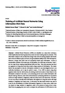
Figure 1: Solve XOR (2-2-1) problem Using OBPM and BPM 4.1.2 Solve XOR (2-2-1) problem using Seven Algorithms: In this experiment, seven different algorithms have been compared in term of the number of epochs: EVDBD [14], OBPM and OBP [10], while the rest of these algorithms are: DBD [5], QP [2], BPM [18] and BP [18]. (The parameters to solve the XOR (2-2-1) problem for all algorithms mentioned in table 3).
Notice that with the DBD and EVDBD algorithms there is no constant value for the learning rate, instead the learning rate is initialized with values for each training process as shown in the first column in table 4 then these learning rates values are adapted through the training epochs. Figure 2 represents the previous table. As you can see, the OBPM (with momentum of 0.8) is the fastest proceeded by the EVDBD which is faster than the OBP. Then, comes the DBD with a close number of epochs to the OBP. According to the last three algorithms which took a larger number of epochs, they are the QP, BPM and BP respectively. As seen in table 3, the OBP and OBPM took
10000
BP BPM 0.8
9000
QP 8000
DBD OBP
7000
EVDBD MSE
6000
OBPM 0.8
5000 4000 3000 2000 1000 0 0.1
0.2
0.3
0.4
0.5
0.6
0.7
0.8
0.9
1
Learning Rate
Figure 2: Solve XOR (2-2-1) problem using Seven Algorithms
4.2 Optical Character Recognition problem In this section, the following algorithms; OBPM and BPM are implemented. In addition, three neural networks are developed and trained to recognize handwritten characters. Two algorithms were used, BPM and OBPM for the first two networks, while only OBPM were used to test the last network because the standard algorithm takes too long time to trains and the comparative is insufficient.
4.2.1 48-8- 4 OCR Problems
hidden and output units, and 0.1 for momentum factor, and binary input values were used [0, 1].
4.2.1.1 48-8- 4 OCR Problems without Biases This network was trained without momentum factor in [12]. As shown in table 5, comparison results of standard BPM algorithm and proposed OBPM algorithm are made using different learning rates. The first column represents the learning rate. Experiment results for the 48-8-4 OCR without biases for the two algorithms. Max, Min and Avg. are the maximum, minimum and the average of number of epochs, respectively. S.D. is the standard deviation of the number of epochs. Remember that the number of trials is 20 with each learning rate. Table 5: Results for OCR problem without biases η Algo. Max Min Avg S.D. BPM 20647 2283 7454.2 7481.4 63 11 22.8 15.3 0.1 OBPM BPM 10252 1145 3252.8 3275.3 28 6 11.6 5.7 0.2 OBPM 4940 764 1639.43 1334.5 BPM 18 4 10.05 8.2 0.3 OBPM 2548 576 1063.7 819.7 BPM 9 2 5.1 1.8 0.4 OBPM As shown in the table 5 and figure 3, a huge decrease in the number of required training epochs is obtained using the OBPM. It should be noted that, out of 20 experiments with learning rate equal to 0.4, the network needs only 2 epochs to train in 4 trials. Max
70
Min
60
Avg
50
Epochs
less number of parameters (which are problem dependent); besides the two of them are speeding up the training process. Here comes the trade-off between speed up the training process and the number of parameters which varies from one problem to another, so the best algorithm here is the OBPM.
40 30 20
This experiment refers to the training of multilayer feedforward neural networks to recognizing 8x6 pixel handwritten character from A to J. The network has 48 input units, 8 hidden units, and 4 output units (which represent the output of each character in binary code (e.g. output for A is 0000, and J is 1001)).
10
Twenty experiment runs were performed with each learning rate and with random initial weights setting over the interval [-0.5, 0.5]. All training processes discontinued when the MSE becomes less than or equal to 0.0001.
25000
0 1.0
2.0
3.0
4.0
Learning Rate
(a) Max Min
Epochs
20000
Avg
15000 10000 5000
The proposed algorithm OBPM and BPM were tested in optical character recognition problem (OCR) using two network architectures .The first network consists of 48-84 without biases and constant momentum was set to 0.3. The bipolar input values were used [-1, 1], while the second network has the same structure but with biases for
0 1.0
2.0
3.0
4.0
Learning Rate
(b) Figure 3: results for OCR problem without biases (a) Using OBPM (b) Using BPM
(b)
4.2.1.2 48-8-4 OCR Problem with Biases As shown in table 6, comparison results between the standard BPM algorithm and proposed OBPM algorithm are made using different learning rates. Experiment results for the 48-8-4 OCR with biases for the two algorithms and momentum factor equal to 0.1. The binary input values were used [0, 1]. Table 6: Results for OCR problem with biases η Algo. Max Min Avg S.D. BPM 69006 52704 62121.7 6507.1 380 400.5 22 0.1 OBPM 423 BPM 77170 25330 32862.3 12754.1 195 349.8 244.5 0.2 OBPM 327 BPM 40328 17006 21108.75 5900.9 145 202.67 156.1 0.3 OBPM 155 BPM 22024 11143 15765.3 3102.5 107 257.2 211.2 0.4 OBPM 220 As shown in the table 6 and figure 4, there are huge differences in the number of required training epochs using the OBPM and BPM algorithms. Notice that, out of 20 experiments with learning rate equal to 0.4, the network needed 107 epochs to train in 3 experiments, while BPM needed to 11143 epochs. Max 500
Min
Epochs
400
Avg
300 200 100 0 0.1
0.2
0.3
0.4
Learning Rate
4.2.2 Solve OCR problem (96-24-4 with training set size =100 and noise rate equals to 4%) Using OBPM and BPM The architecture of the network that has been used in this experiment is 96-24-4 and the value of learning rate from 0.1 to 0.4. We used momentum equals to 0.2; the aim of this training process is dealing with a large training set size where the used size here was 100 patterns. Each character has been written ten times through ten different writers. Beside, we have focused on studying the effect of the noise on the inputs with OBPM. We added the average of noise about 4% per each pattern. The results of this experiment were presented in the following table. Table 7: Solve OCR problem (96-24-4 with training set size =100 and noise rate equals to 4%) Using OBPM and BPM
OBPM BPM
0.1
23
498
0.2
24
370
0.3
38
283
0.4
42
209
From the previous table, it can see that the OBPM was able to solve this problem, inspite of the large size of training set and the noise for each character. The note that it should mention here is that using a small learning rate with such problems may be better. Whereas with the BPM if the learning rate increases, then the required number of epochs will reduce. It will also assure that whenever the size of the training set increased, the number of required epochs gradually and obviously becomes less using BPM. Despite that, the OBPM still achieves better than the BPM and has the ability to generalize.
(a) Max 100000
Min
Epochs
80000
4.2.3 Solve OCR Problem (10000-L-M neural network)
Avg
60000 40000 20000 0 0.1
0.2
0.3
0.4
Learning Rate
(b) Figure 4: results for OCR problem with biases (a) Using OBPM (b) Using BPM
From the previous experiments, different sizes have been examined for input layer, but in this test the size of the input layer has been maximized to be compatible with real problems. Each character has been represented with 100 rows and 100 columns, so that the size of the input layer becomes very large which is 10000 units. The inputs of this network are binary with biases. The training for each network proceeded till the MSE becomes 0.0001 through different learning rates.
4.2.3.1 Solve OCR Using OBPM:
problem
(10000-L-4)
This network has been constructed to recognize the characters from A-J with different sizes of hidden layer
40, 50, and 60 units with many learning rates. The next table represents the results of this network:
Table 10: Solve OCR problem (10000-L-6) Using OBPM HLS
Table 8: Solve OCR problem (10000-L-4) Using OBPM
80 90 100
HLS
0.1 97 65 47
40 50 60
0.2 61 49 38
0.3 43 40 26
0.4 39 22 24
HLS refers to Hidden layer size. The row that represents the hidden layer size equals to 60 is the best row but it should say that using hidden layer size greater than 60 will prevent the network from generalization. So using a medium hidden layer size is better for generalization and acceleration of the training process.
4.2.3.2 Solve OCR Using OBPM:
problem
(10000-L-5)
The new thing about this experiment is maximizing the output layer and that is to help this network to recognize the charters from A-Z (for example, the target output for the character A is 00000, and for Z is 11001). The number of units (L) in the hidden layer was 30, 40, 50, 60, 70 and 80 units. The following table summarizes the results of this experiment. The number of epochs that have been put in the table gave a better result from the five trails that have been got with each hidden layer using a certain learning rate. Table 9: Solve OCR problem (10000-L-5) Using OBPM HLS 30 40 50 60 70 80
0.1 150 110 84 80 60 53
0.2 71 71 54 37 30 24
0.3 70 60 37 31 26 23
0.4 54 36 32 28 26 22
From the previous, it can notice that OBPM could solve this problem too and through the different sizes of hidden layer. For this test and the previous tests using hidden layer size of 60 and 70 is better because it is close to the results of hidden layer size equals to 80, but it reduces from falling into local minima or overfitting.
4.2.3.3 Solve OCR Using OBPM:
problem
(10000-L-6)
The aim of this network is recognizing a large number of symbols. The size of the output layer has been maximized to 6. So this network has the ability to recognize the capital letters from A-Z, small letters from a-z beside the digits from 0-9. According to the size of the hidden layer it was 80, 90 and 100 units as in the following table:
0.1 73 50 32
0.2 66 50 26
0.3 41 38 21
From the results of the previous table, the new result is that when the size of the training set (i.e. number of symbols) increases it becomes very important to use a larger size of the hidden layer. In addition, the required number of epochs becomes less. Note: we have not concentrated on the comparison between OBPM and BPM in the last three experiments. That is because; to train the network that have the architecture 10000-30-5 (that is to recognize characters from A-Z) with learning rate 0.1 with the same conditions. we got the following results: -
OBPM needed 151 epochs.
-
BPM needed 15600 epochs and more than 20 hours training on Dell machine (Pentium IV).
5 Conclusion This paper introduced a proposed algorithm OBPM which is an enhanced version of the BPM algorithm, which is used to train the multilayer neural networks. The study has shown that OBPM is much faster and can speed up the training process. The experiment results confirmed these observations. The new approach has been applied on different: (architectures, input vectors (bipolar, binary), momentum factor, biases and learning rate) and it has shown tangible improvements. The use of a momentum term with OBP accelerates the training process of neural networks. The algorithm was superior to other methods in terms of requiring less number of epochs to converge as well as less parameters are used (i.e. it does not uses many parameters which problem dependent like many algorithms mentioned above).
References: [1] Carling, A., Alison, Back Propagation. Introducing Neural Networks, 1992, 133-154. [2] Fahlman, S. E., Faster-learning variations on Backpropagation: an empirical study. Proceedings of the 1988 Connectionist Models Summer School, 3851. [3] Freeman, J. A., Skapura, D. M., Backpropagation. Neural Networks Algorithm Applications and Programming Techniques, 1992, 89-125.
[4] F. M. Silva and L. B. Almeida,”Speeding up backpropagation”, in Advanced Neural Computers, 1990,151-158. [5] Jacobs, R. A., Increased rates of convergence through learning rate adaptation, Neural Networks, 1988,1,169-180 [6] J. Leonard and M. A. Kramer, “Improvement of the backpropagation algorithm for training neural networks”, Computer Chem. Engng., 1990, 14(3),337-341. [7] Martin T. Hagan, Howard B. Demuth, Neural Networks Design, 1996, 11.1-12.52 [8] Maureen Caudill, and Charles Butler, Understanding Neural Networks: Computer Explorations, Volume 1,1993,.155-218 [9] Minai, A.A., Williams, R.D., Acceleration of backpropagation through learning rate momentum adaptation, Proceedings of the International Joint Conference on Neural Networks, 1990, 1676-1679. [10] M.A. Otair and W.A. Salameh, An Improved BackPropagation Neural Networks using a Modified Nonlinear Function, Proceedings of the IASTED International Conference, 2004,442-447 [11] M.A. Otair and W.A. Salameh,” Speeding Up Backpropagation Neural Networks”, under preparation, 2004. [12] M.A. Otair and W.A. Salameh, Online Handwritten Character Recognition Using An Optical Backpropagation Neural Networks, Proceedings of The 2004 International Research Conference on Innovations in Information Technology, 2004, 334341. [13] M.A. Otair and W.A. Salameh,” Solving The Exclusive-OR Problem Using an Optical Backpropagation Algorithm”, under preparation, 2004. [14] M.A. Otair and W.A. Salameh, Enhanced Version of Delta-Bar-Delta, under preparation, 2004. [15] M. Hagiwara,”Theoretical derivation of momentum term in backpropagation”, in Int. Joint Conf. On Neural Networks, 1992,682-686. [16] Riedmiller, M and Braun, H., A direct adaptive method for faster backpropagation learning the PROP algorithm. Proceedings of the IEEE international conference on Neural Networks (ICNN), Vol. I, San Francisco, CA, ,1993, 586-591. [17] Robert Callan, The Essence of Neural Networks, Southmpton Institute, 1999, 33-52. [18] Rumelhart, D. E., Hinton, G. E., and Williams, R. J., Learning internal representations by error propagation, In D. E. Rumelhart and J. L. McClelland (eds) Parallel Distributed Processing, 1986, 318-362. [19] Rumelhart, D. E., Richard Durbin, Richard Golden, and Yves Chauvin, Backpropagation: theoretical foundations. In Y.Chauvin and D. E Rumelhart (eds). Backpropagation and Connectionist Theory. Lawrence Erlbaum, 1992. [20] Simon Hakin , Neural Networks A Comprehensive Foundation ,2nd Edition , 1999 ,161-184
[21] T. M. Mitchell, “Machine Learning (McGraw Hill, Boston, MA), 1997,p.119 [22] T. Tollenaere, “SuperSAB: Fast adaptive backpropagation with good scaling properties”, Neural Networks, 1990,3,561-573. [23] W. Schiffmann, M. Joost and R Werner, “ Comparison of optimized backprop algorithms”, Artificial Neural Networks European Symposium, 1993. [24] X. H. Yu and G.A. Chen, ”Efficient estimation of dynamically optimal learning rate and momentum for backpropagation learning”, in Proc. of IEEE ICNN95, 1995,385-88. [25] Y Dali and L Zemin,”A LMS algorithm with stochastic momentum factor”, in Proc. of ISCAS-93, 1993, 1250-1253.