Efficiently Solving Quantified Bit-Vector Formulas - Leonardo de Moura

Efficiently Solving Quantified Bit-Vector Formulas Christoph M. Wintersteiger

Youssef Hamadi

Leonardo de Moura

Computer Systems Institute ETH Zurich Zurich, Switzerland [email protected]

Microsoft Research Cambridge 7 JJ Thomson Avenue Cambridge CB3 0FB, UK [email protected]

Microsoft Research Redmond One Microsoft Way Redmond, WA, 98074, USA [email protected]

Abstract—In recent years, bit-precise reasoning has gained importance in hardware and software verification. Of renewed interest is the use of symbolic reasoning for synthesising loop invariants, ranking functions, or whole program fragments and hardware circuits. Solvers for the quantifier-free fragment of bit-vector logic exist and often rely on SAT solvers for efficiency. However, many techniques require quantifiers in bit-vector formulas to avoid an exponential blow-up during construction. Solvers for quantified formulas usually flatten the input to obtain a quantified Boolean formula, losing much of the word-level information in the formula. We present a new approach based on a set of effective word-level simplifications that are traditionally employed in automated theorem proving, heuristic quantifier instantiation methods used in SMT solvers, and model finding techniques based on skeletons/templates. Experimental results on two different types of benchmarks indicate that our method outperforms the traditional flattening approach by multiple orders of magnitude of runtime.

I. I NTRODUCTION The complexity of integrated circuits continues to grow at an exponential rate and so does the size of the verification and synthesis problems arising from the hardware design process. To tackle these problems, bit-precise decision procedures are a requirement and oftentimes the crucial ingredient that defines the efficency of the verification process. Recent years also saw an increase in the utility of bitprecise reasoning in the area of software verification where low-level languages like C or C++ are concerned. In both areas, hardware and software design, methods of automated synthesis (e.g., LTL synthesis [23]) become more and more tangible with the advent of powerful and efficient decision procedures for various logics, most notably SAT and SMT solvers. In practice, however, synthesis methods are often incomplete, bound to very specific application domains, or simply inefficient. In the case of hardware, synthesis usually amounts to constructing a module that implements a specification [23], [20], while for software this can take different shapes: inferring program invariants [16], finding ranking functions for termination analysis [28], [24], [8], program fragment synthesis [26], or constructing bugfixes following an error-description [27] are all instances of the general synthesis problem. In this paper, we present a new approach to solving quantified bit-vector logic. This logic allows for a direct mapping of hardware and (finite-state) software verification problems and

is thus ideally suited as an interface between the verification or synthesis tool and the decision procedure. In many practically relevant applications, support for uninterpreted functions is not required and if this is the case, quantified bit-vector formulas can be reduced to quantified Boolean formulas (QBF). In practice however, QBF solvers face performance problems and they are usually not able to produce models for satisfiable formulas, which is crucial in synthesis applications. The same holds true for many automated theorem provers. SMT solvers on the other hand are efficient and produce models, but usually lack complete support for quantifiers. The ideas in this paper combine techniques from automated theorem proving, SMT solving and synthesis algorithms. We propose a set of simplifications and rewriting techniques that transform the input into a set of equations that an SMT solver is able to solve efficiently. A model finding algorithm is then employed to refine a candidate model iteratively, while we use function or circuit templates to reduce the number of iterations required by the algorithm. Finally, we evalutate a prototype implementation of our algorithm on a set of hardware and software benchmarks, which indicate speedups of up to five orders of magnitude compared to flattening the input to QBF. II. BACKGROUND We will assume the usual notions and terminology of first order logic and model theory. We are mainly interested in many-sorted languages, and bit-vectors of different sizes correspond to different sorts. We assume that, for each bitvector sort of size n, the equality =n is interpreted as the identity relation over bit-vectors of size n. The if-then-else (multiplexer) bit-vector term ite n is interpreted as usual as ite(true, t, e) = t and ite(false, t, e) = e. As a notational convention, we will always omit the subscript. We call 0arity function symbols constant symbols, and 0-arity predicate symbols propositions. Atoms, literals, clauses, and formulas are defined in the usual way. Terms, literals, clauses and formulas are called ground when no variable appears in them. A sentence is a formula in which free variables do not occur. A CNF formula is a conjunction C1 ∧ . . . ∧ Cn of clauses. We will write CNF formulas as sets of clauses. We use a, b and c for constants, f and g for function symbols, p and q for predicate symbols, x and y for variables, C for clauses, ϕ for formulas, and t for terms. We use x: n to denote that

variable x is a bit-vector of size n. When the bit-vector size is not specified, it is implicitly assumed to be 32. We use f : n1 , . . . , nk → nr to denote to denote that function symbol f has arity k, argument bit-vectors have sizes n1 , . . . , nk , and the result bit-vector has size nr . We use ϕ[x1 , . . . , xn ] to denote a formula that may contain variables x1 , . . . , xn , and similarily t[x1 , . . . , xn ] is defined for a term t. Where there is no confusion, we denote ϕ[x1 , . . . , xn ] by ϕ[x] and t[x1 , . . . , xn ] by t[x]. In the rest of this paper, the difference between functions and predicates is trivial, and we will thus only discuss functions except at a few places. We use the standard notion of a structure (interpretation). A structure that satisfies a formula F is said to be a model for F . A theory is a collection of first-order sentences. Interpreted symbols are those symbols whose interpretation is restricted to the models of a certain theory. We say a symbol is free or uninterpreted if its interpretation is not restricted by a theory. We use BitVec to denote the bit-vector theory. In this paper we assume the usual interpreted symbols for bit-vector theory: +n , ∗n , concat m,n , ≤n , 0n , 1n , . . . . Where there is no confusion, we omit the subscript specifying the actual size of the bit-vector. A formula is satisfiable if and only if it has a model. A formula F is satisfiable modulo the theory BitVec if there is a model for {F } ∪ BitVec. III. Q UANTIFIED B IT-V ECTOR F ORMULAS A Quantified Bit-Vector Formula (QBVF) is a many sorted first-order logic formula where the sort of every variable is a bit-vector sort. The QBVF-satisfiability problem, is the problem of deciding whether a QBVF is satisfiable modulo the theory of bit-vectors. This problem is decidable because every universal (existental) quantifier can be expanded into a conjunction (disjunction) of potentially exponential, but finite size. A distinguishing feature in QBVF is the support for uninterpreted function and predicate symbols. Example 1: Arrays can be easily encoded in QBVF using quantifiers and uninterpreted function symbols. In the following formula, the uninterpreted functions f and f ′ are used to represent arrays from bit-vectors of size 8 to bit-vectors of the same size, and f ′ is essentially the array f updated at position a + 1 with value 0: f ′ (a + 1) = 0 ∧ (∀x : 8. x = a + 1 ∨ f ′ (x) = f (x)) . Quantified Boolean formulas (QBF) are a generalization of Boolean formulas, where quantifiers can be applied to each variable. Deciding a QBF is a PSPACE-complete problem. Note that any QBF problem can be easily encoded in QBVF by using bit-vectors of size 1. The converse is not true, QBVF is more expressive than QBF. For instance, uninterpreted function symbols can be used to simulate non-linear quantifier prefixes. The EPR fragment of first-order logic comprises formulas of the form ∃∗ ∀∗ ϕ, where ϕ is a quantifier-free formula with predicates but without function symbols. EPR is a decidable fragment because the Herbrand universe of a

EPR formula is always finite. The satisfiability problem for EPR is NEXPTIME-complete. Theorem 1: The satisfiability problem for QBVF is NEXPTIME-complete.1 QBVF can be used to compactly encode many practically relevant verification and synthesis problems. In hardware verification, a fixpoint check consists in deciding whether k unwindings of a circuit are enough to reach all states of the system. To check this, two copies of the k unwindings are used: Let T [x, x′ ] be a formula encoding the transition relation and I[x] a formula encoding the initial states of a circuit. Furthermore, we define k

′

T [x, x ] ≡ T [x, x0 ] ∧

k−1 ^

T [xi−1 , xi ] ∧ T [xk−1 , x′ ] .

i=1

Then a fixpoint check for k unwindings corresponds to the QBV formula ∀x, x′ . I[x] ∧ T k [x, x′ ] → ∃y, y ′ .I[y] ∧ T k−1 [y, y ′ ] , where x, x′ , y, and y ′ are (usually large) bit-vectors. Of renewed interest is the use of symbolic reasoning for synthesing code [26], loop invariants [7], [16] and ranking functions [8] for finite-state programs. All these applications can be easily encoded in QBVF. To illustrate these ideas, consider the following abstract program: pre while (c) { T } post In the loop invariant synthesis problem, we want to synthesise a predicate I that can be used to show that post holds after execution of the while-loop. Let, pre[x] be a formula encoding the set of states reachable before the beginning of the loop, c[x] be the encoding of the entry condition, T [x, x′ ] be the transition relation, and post [x] be the encoding of the property we want to prove. Then, a suitable loop invariant exists if the following QBV formula is satisfiable. ∀x. pre[x] → I(s) ∧ ∀x, x′ . I(x) ∧ c[x] ∧ T [x, x′ ] → I(x′ ) ∧ ∀x. I(x) ∧ ¬c[x] → post [x] An actual invariant can be extracted from any model that satisfies this formula. Similarly, in the ranking function synthesis problem, we want to synthesise a function rank that decreases after each loop iteration and that is bounded from below. The idea is to use this function to show that a particular loop in the program always terminates. This problem can be encoded as the following QBVF satisfiability problem. ∀x. rank (x) ≥ 0 ∧ ∀x, x′ . c[x] ∧ T [x, x′ ] → rank (x′ ) < rank (x) Note that the general case of this encoding requires uninterpreted functions. The call to rank can not be replaced with an 1 For

a proof of this theorem, see Appendix A.

existentially quantified variable, as it is impossible to express the correct variable dependencies in a linear quantifier prefix. IV. S OLVING QBVF In this section, we describe a QBVF solver based on ideas from first-order theorem proving, SMT solving and synthesis tools. First, we present a set of simplifications and rewriting rules that help to greatly reduce the size and complexity of typical QBVF formulas. Then, we describe how to check whether a given model satisfies a QBVF and how to use this to construct new models, using templates to speed up the process (sometimes exponentially). A. Simplifications & Rewriting Modern first-order theorem provers spend a great part of their time in simplifying/contracting operations. These operations are inferences that remove or modify existing formulas. Our QBV solver implements several simplification/contraction rules found in first-order provers. We also propose new rules that are particularly useful in our application domain. 1) Miniscoping: Miniscoping is a well-known technique for minimizing the scope of quantifiers [17]. We apply it after converting the formula to negation normal form. The basic idea is to distribute universal (existential) quantifiers over conjunctions (disjunctions). This transformation is particularly important in our context because it increases the applicability of rules based on rewriting and macros. We may also limit the scope of a quantifier if a sub-formula does not contain the quantified variable. That is, (∀x.F [x] ∨ G) =⇒ (∀x.F [x]) ∨ G when G does not contain x. We use a similar rule for existential quantifiers over disjunctions. 2) Skolemization: Similarly to first-order theorem provers, in our solver, existentially quantified variables are eliminated using Skolemization. A formula ∀x. ∃y. ¬p(x)∨q(x, y) is converted into the equisatisfiable formula ∀x. ¬p(x)∨q(x, fy (x)), where fy is a fresh function symbol. 3) A conjunction of universally quantified formulas: After NNF conversion, miniscoping and skolemization. The QBV formula is written as a conjunction of universally quantified formulas: (∀x. ϕ1 [x]) ∧ . . . ∧ (∀x. ϕn [x]). This form is very similar to that used in first-order theorem provers. However, we do not require each ϕi [x] to be a clause. 4) Destructive Equality Resolution (DER): DER allows us to solve a negative equality literal by simply applying the following transformation: (∀x, y. x 6= t ∨ ϕ[x, y]) =⇒ (∀y. ϕ[t, y]) , where t does not contain x. For example, using DER, the formula ∀x, y. x 6= f (y) ∨ g(x, y) ≤ 0 is simplified to ∀y. g(f (y), y) ≤ 0. DER is essentially an equality substitution rule. This becomes clear when we write the clause on the lefthand-side using an implication: ∀x, y. x = t → ϕ[x, y]. It is straightforward to implement DER; a naive implementation eliminates a single variable at a time. In our experiments,

we observed this naive implementation was a bottleneck in benchmarks where hundreds of variables could be eliminated. The natural solution is to eliminate as many variables simultaneously as possible. The only complication in this approach is that some of the variables being eliminated may depend on each other. We say a variable x directly depends on y in DER, when there is a literal x 6= t[y]. In general we are presented with a formula of the following form: ∀x1 , . . . , xn , y. x1 6= t1 ∨ . . . ∨ xn 6= tn ∨ ϕ[x1 , . . . , xn , y] , where each xi may depend on variables xj , j 6= i. First, we build a dependency graph G where the nodes are the variables xi , and G contains an edge from xi to xj whenever xj depends on xi . Next, we perform a topological sort on G, and whenever a cycle is detected when visiting node xi , we remove xi from G and move xi 6= ti to ϕ[x1 , . . . , xn , y]. Finally, we use the variable order xk1 , . . . , xkm (m ≤ n) produced by the topological sort to apply DER simultaneously. Let θ be a substitution, i.e., a mapping from variables to terms. Initially, θ is empty. For each variable xki we first apply θ to tki producing t′ki , and then update θ := θ ∪ {xki 7→ t′ki }. After all variables xki were processed, we apply the resulting substitution θ to ϕ[x1 , . . . , xn , y]. As a final remark, the applicability of DER can be increased using theory solvers. The idea is to rewrite inequalities of the form t1 [x, y] 6= t2 [x, y], containing a universal variable x, into x 6= t′ [y]. This rewriting step is essentially equivalent to a theory solving step, where t1 [x, y] = t2 [x, y] is solved for x. In the case of linear bit-vector equations, this can be achieved when the coefficient of x is odd [12]. 5) Rewriting: The idea of using rewriting for performing equational reasoning is not new. It traces back to the work developed in the context of Knuth-Bendix completion [21]. The basic idea is to use unit clauses of the form ∀x. t[x] = r[x] as rewrite rules t[x] ; r[x], when t[x] is “bigger than” r[x]. Any instance t[s] of t[x] is then replaced by r[s]. For example, in the formula (∀x. f (x, a) = x) ∧ f (h(b), a) ≥ 0, the quantifier can be used as the rewrite rule f (x, a) ; x. Thus, the term f (h(b), a) ≥ 0 can be simplified to h(b) ≥ 0, producing the new formula (∀x. f (x, a) = x) ∧ h(b) ≥ 0 . We observed that rewriting is quite effective in many QBVF benchmarks, in particular, in hardware fixpoint check problems. Our goal is to use rewriting as an incomplete simplification technique. So, we are not interested in computing critical pairs and generating a confluent rewrite system. First-order theorem provers use sophisticated term orderings to orient the equations t[x] = r[x] (see, e.g., [17]). We found that any term ordering, where interpreted symbols (e.g., +, *) are considered “small”, works for our purposes. This can be realised, for instance, using a Knuth-Bendix Ordering where the weight of interpreted symbols is set to zero. The basic idea of this

heuristic is to replace uninterpreted symbols with interpreted ones. For example, using f (x) ; 2x + 1, we can simplify f (a) − a to 2a + 1 − a, and then apply a bit-vector rewriting rule and reduce it to a + 1. 6) Macros & Quasi-Macros: A macro is a unit clause of the form ∀x. f (x) = t[x], where f does not occur in t. Macros can be eliminated from QBVF formulas by simply replacing any term of the form f (r) with t[r]. Any model for the resultant formula can be extended to a model that also satisfies ∀x. f (x) = t[x]. For example, consider the formula (∀x. f (x) = x + a) ∧ f (b) > b . After macro expansion, this formula is reduced to the equisatisfiable formula b + a > b. The interpretation a 7→ 1, b 7→ 0 is a model for this formula. This interpretation can be extended to f (x) 7→ x + 1, a 7→ 1, b 7→ 0 , which is a model for the original formula. This particular way to represent models is described in more detail in section IV-B. A quasi-macro is a unit clause of the form ∀x.f (t1 [x], . . . , tm [x]) = r[x] , where f does not occur in r[x], f (t1 [x], . . . , tm [x]) contains all x variables, and the following system of equations can be solved for x1 , . . . , xn y1 = t1 [x], . . . , ym = tm [x] , where y1 , . . . , ym are new variables. A solution of this system is a substitution θ : x1 7→ s1 [y], . . . , xn 7→ sn [y] . We use the notation ϕ ↓ θ to represent the application of the substitution θ to the formula ϕ. Then, the quasi-macro can be replaced with the macro ^ ∀y.f (y) = ite( yi = ti [x], r[x], f ′ (y)) ↓ θ i ′

where f is a fresh function symbol. Intuitively, the new formula is saying that when the arguments of f are of the form ti [x], then the result should be r[x], otherwise the value is not specified. Now, the quasi-macro was transformed into a macro, the quantifier can be eliminated using macro expansion. Example 2 (Quasi-Macro): ∀x.f (x + 1, x − 1) = x is a quasi-macro, because the system y1 = x + 1, y2 = x − 1 can be solved for x. A possible solution is the substitution θ = {x 7→ y1 − 1}. Thus, we can transform this quasi-macro into the macro: ∀y1 , y2 . f (y1 , y2 ) = ite(y1 = x + 1 ∧ y2 = x − 1, x, f ′ (y1 , y2 )) ↓ θ After applying the substitution θ and simplifying the formula, we obtain ∀y1 , y2 . f (y1 , y2 ) = ite(y2 = y1 − 2, y1 − 1, f ′ (y1 , y2 )) . In our experiments, we observed that the solvability condition is trivially satisfied in many instances, because all variables x

are actual arguments of f . Assume that variable xi is the ki -th argument of f . Then, the substitution θ is of the form {x1 7→ yk1 , . . . , xn 7→ ykn }. For example, i n many benchmarks we found quasi-macros that are bigger versions of ∀x1 , x2 . f (x1 , x1 + x2 , x2 ) = r[x1 , x2 ] . 7) Function Argument Discrimination (FAD): We have observed that after applying DER the i-th argument of many function applications is always a bit-vector value such as: 0, 1, 2, etc. For any function symbol f and QBV formula ϕ, the following macro can be conjoined with ϕ while preserving satisfiability: ∀x, y. f (x, y) = ite(x = v, fv (y), f ′ (x, y)) , where fv and f ′ are fresh function symbols, and v is a bitvector value. Now, suppose that the first argument of all f applications are bit-vector values. The macro above will reduce f (v ′ , t) to fv (t) when v = v ′ , and f ′ (v ′ , t) otherwise. The transformation can be applied again to the f ′ applications if their first argument is again a bit-vector value. Example 3 (FAD): Let ϕ be the formula (∀x. f (1, x, 0) ≥ x) ∧ f (0, a, 1) < f (1, b, 0) ∧ f (0, c, 1) = 0 ∧ c = a. Applying FAD twice (for the values 0 and 1) on the first argument of f , we obtain (∀x. f1 (x, 0) ≥ x) ∧ f0 (a, 1) < f1 (b, 0) ∧ f0 (c, 1) = 0 ∧ c = a. Applying FAD for the third argument of f1 and f0 results in (∀x. f1,0 (x) ≥ x) ∧ f0,1 (a) < f1,0 (b) ∧ f0,1 (c) = 0 ∧ c = a. Since FAD is based on macro definitions, the infrastructure used for constructing interpretations for macros may be used to build an interpretation for f based on the interpretations of f1,0 and f0,1 . 8) Other simplifications: As many other SMT solvers for bit-vector theory ([6], [5], [2]), our QBVF solver implements several bit-vector specific rewriting/simplification rules such as: a − a =⇒ 0. These rules have been proved to be very effective in solving quantifier-free bit-vector benchmarks, and this is also the case for the quantified case. From now on, we assume there is a procedure Simplify that given a QBV formula ϕ, converts it into negation normal form, then applies miniscoping, skolemization, and then applies the other simplification described in this section up to saturation. B. Model Checking Quantifiers Given a structure M , it is useful to have a procedure MC that checks whether M satisfies a universally quantified formula ϕ or not. We say MC is a model checking procedure. Before we describe how MC can be constructed, let us take a look at how structures are encoded in our approach. We use BV to denote the structure that assigns the usual interpretation to

the (interpreted) symbols of the bit-vector theory (e.g., +, ∗, concat , etc). In our approach, the structures M are based on BV . We use |BV |n to denote the interpretation of the sort of bit-vectors of size n. With a small abuse of notation, the elements of |BV |n are {0n , 1n , . . . , 2nn−1 }. Again, where there is no confusion, we omit the subscript. The interpretation of an arbitrary term t in a structure M is denoted by M [[t]], and is defined in the standard way. We use M {x 7→ v} to denote a structure where the variable x is interpreted as the value v, and all other variables, function and predicate symbols have the same interpretation as in M . That is, M {x 7→ v}(x) = v. For example, BV {x 7→ 1}[[2 ∗ x + 1]] = 3. As usual, M {x 7→ v} denotes M {x1 7→ v1 }{x2 7→ v2 } . . . {xn 7→ vn }. For each uninterpreted constant c that is a bit-vector of size n, the interpretation M (c) is an element of |BV |n . For each uninterpreted function (predicate) f : n1 , . . . , nk → nr of arity k, the interpretation M (f ) is a term tf [x1 , . . . , xk ], which contains only interpreted symbols and the free variables x1 : n1 , . . . , xk : nk . The interpretation M (f ) can be viewed as a function definition, where for all v in |BV |n1 × . . . × |BV |nk , M (f )(v) = BV {x 7→ v}[[tf [x]]]. Example 4 (Model representation): Let ϕa be the following formula: (∀x. ¬(x ≥ 0) ∨ f (x) < x) ∧ (∀x. ¬(x < 0) ∨ f (x) > x + 1) ∧ f (a) > b ∧ b > a + 1 . Then the interpretation Ma := {f (x) 7→ ite(x ≥ 0, x − 1, x + 3), a 7→ −1, b 7→ 1} is a model for ϕa . For instance, we have M [[f (a)]] = 2. Usually, SMT solvers represent the interpretation of unintepreted function symbols as finite function graphs (i.e., lookup tables). A function graph is an explicit representation that shows the value of the function for a finite (and relatively small) number of points. For example, let the function graph {0 7→ 1, 2 7→ 3, else 7→ 4} be the interpretation of the function symbol g. It states that the value of the function g at 0 is 1, at 2 it is 3, and for all other values it is 4. Any function graph can be encoded using ite terms. For example, the function graph above can be encoded as g(x) 7→ ite(x = 0, 1, ite(x = 2, 3, 4)). Our approach for enconding interpretations is symbolic and potentially allows for an exponentially more succinct representation. For example, assuming f is a function from bit-vectors of size 32, the interpretation f (x) 7→ ite(x ≥ 0, x − 1, x + 3) would correspond to a very large function graph. When models are encoded in this fashion, it is straightforward to check whether a universally quantified formula ∀x. ϕ[x] is satisfied by a structure M [13]. Let ϕM [x] be the formula obtained from ϕ[x] by replacing any term f (r) with M [[f (r)]], for every uninterpreted function symbol f . A structure M satisfies ∀x. ϕ[x] if and only if ¬ϕM [s] is unsatisfiable, where s is a tuple of fresh constant symbols.

Example 5: For instance, in Example 4, the structure Ma satisfies ∀x. ¬(x ≥ 0) ∨ f (x) < x because s ≥ 0 ∧ ¬(ite(s ≥ 0, s − 1, s + 3) < s) is unsatisfiable. Let Mb be a structure identical to Ma in Example 4, but where the interpretation Mb (f ) of f is x + 2. Mb does not satisfy ∀x. ¬(x ≥ 0) ∨ f (x) < x in ϕa because the formula s ≥ 0 ∧ ¬(s + 2 < s) is satisfiable, e.g., by s 7→ 0. The assignment s 7→ 0 is a counter-example for Mb being a model for ϕa . The model-checking procedure MC expects two arguments a universally quantified formula ∀x. ϕ[x] and a structure M . It returns ⊤ if the structure satisfies ∀x. ϕ[x], and a non-empty finite set V of counter-examples otherwise. Each counter-example is a tuple of bit-vector values v such that M {x 7→ v}[[ϕ[x]]] evaluates to false. C. Template Based Model Finding In principle, the verification and synthesis problems described in section III can be attacked by any SMT solver that supports universally quantified formulas, and that is capable of producing models. Unfortunately, to the best of our knowledge, no SMT solver supports complete treatment of universally quantified formulas, even if the variables range over finite domains such as bit-vectors. On satisfiable instances, they will often not terminate or give up. On some unsatisfiable instances, SMT solvers may terminate using techniques based on heuristic-quantifier instantiation [9]. It is not surprising that standard SMT solvers cannot handle these problems; the search space is simply too large. Synthesis tools based on automated reasoning try to constrain the search space using templates. For example, when searching for a ranking function, the synthesis tool may limit the search to functions that are linear combinations of the input. This simple idea immediately transfers to QBVF solvers. In the context of a QBVF solver, a template is just an expression t[x, c] containing free variables x, interpreted symbols, and fresh constants c. Given a tuple of bit-vector values v, we say t[x, v] is an instance of the template t[x, c]. A template can also viewed as a parametric function definition. For example, the template ax+b, where a and b are fresh constants, may be used to guide the search for an interpretation for unary function symbols. The expressions x + 1 (a 7→ 1, b 7→ 1) and 2x (a 7→ 2, b 7→ 0) are instances of this template. We say a template binding for a formula ϕ is a mapping from uninterpreted function (predicate) symbols fi , occurring in ϕ, to templates ti [x, c]. Conceptually, one template per uninterpreted symbol is enough. If we want to consider two different templates t1 [x, c1 ] and t2 [x, c2 ] for an uninterpreted symbol f , we can just combine them in a single template t′ [x, (c1 , c2 , c)] ≡ ite(c = 1, t1 [x, c1 ], t2 [x, c2 ]), where c is a new fresh constant. This approach can be extended to construct templates that are combinations of smaller “instructions” that can be combined to construct a template for the desired class of functions.

Without loss of generality, let us assume that ϕ contains only one uninterpreted function symbol f . So, a template based model finder is a procedure TMF that given a ground formula ϕ and a template binding TB = {f 7→ t[x, c]}, returns a structure M for ϕ s.t. the interpretation of f is t[x, v] for some bit-vector tuple v if such a structure exists. TMF returns ⊥ otherwise. Since we assume ϕ is a ground formula, a standard SMT solver can be used to implement TMF. We just need to check whether ^ f (r) = t[r, c] ϕ∧

solver(ϕ, TB) ϕ := Simplify(ϕ) w.l.o.g. assume ϕ is of the form ∀x. φ[x] ρ := HeuristicInst(φ[x]) loop if SMT(ρ) = unsat return unsat M := TMF(ρ, TB) if M = ⊥ return unsat modulo TB V := MC(ϕ, M ) if V = ⊤Vreturn (sat, M ) ρ := ρ ∧ v∈V φ[v]

f (r)∈ϕ

is satisfiable. If this is the case, the model produced by the SMT solver will assign values to the fresh constants c in the template t[x, c]. When TMF(ϕ, TB) succeeds we say ϕ is satisfiable modulo TB. Example 6 (Template Based Model Finding): Let ϕ be the formula f (a1 ) ≥ 10 ∧ f (a2 ) ≥ 100 ∧ f (a3 ) ≥ 1000 ∧ a1 = 0 ∧ a2 = 1 ∧ a3 = 2 and the template binding TB be {f 7→ c1 x + c2 }. Then, the corresponding satisfiability query is: f (a1 ) ≥ 10 ∧ f (a2 ) ≥ 100 ∧ f (a3 ) ≥ 1000 ∧ a1 = 0 ∧ a2 = 1 ∧ a3 = 2 ∧ f (a1 ) = c1 a1 + c2 ∧ f (a2 ) = c1 a2 + c2 ∧ f (a3 ) = c1 a3 + c2 The formula above is satisfiable, e.g., by the assignment c1 7→ 1 and c2 7→ 1000. Therefore, ϕ is satisfiable modulo TB. D. Solver Architecture The techniques described in this section can be combined to produce a simple and effective solver for nontrivial benchmarks. Figure 1 shows the algorithm used in our prototype. The solver implements a form of counterexample guided refinement where a failed model-checking step suggests new instances for the universally quantified formula. This method is also a variation of model-based quantifier instantiation [13] based on templates. The procedure SMT is an SMT solver for the quantifier-free bit-vector and uninterpreted function theory (QF UFBV in SMT-LIB [1]). The procedure HeuristicInst(φ[x]) creates an initial set of ground instantes of φ[x] using heuristic instantiation. Note that the formula ρ is monotonically increasing in size, so the procedures SMT and TMF can exploit incremental solving features available in state-of-the-art SMT solvers. Theorem 2: The algorithm in Figure 1 is complete modulo the given template TB.2 The algorithm in Figure 1 is complete for QBVF if TMF never fails, that is, M is never ⊥. This can be accomplished using a template that simply covers all relevant functions: Let us assume w.l.o.g that every function in ϕ has only one 2 For

a proof of this theorem, see Appendix B.

Fig. 1.

QBVF solving algorithm.

argument and it is a bit-vector of size 2n . Then, using the template ite(x = c1 , a1 , . . . , ite(x = c2n −1 , a2n −1 , a2n ) . . .) guarantees that TMF will never fail, where c1 , . . . c2n −1 , a1 , . . . , a2n are the template parameters. Of course, it is impractical to use this template in practice. Therefore, in our implementation, we consider templates of increasing complexity. We essentially use an outer-loop that automatically increases the size of the templates whenever the inner-loop returns unsat modulo TB. In many cases, using actual tuples of bit-vector values is not the best strategy for instantiating quantifers. For example, assume f is a function from bit-vectors of size 32 to bit-vectors of the same size in (∀x. f (x) ≥ 0), f (a) < 0 . To prove this formula to be unsatisfiable, we should instantiate the quantifier with a instead of the 232 possible bit-vector values. Therefore, we use an approach similar to the one used in [13]. Given a tuple (v1 , . . . , vn ) in V , if there is a term t in ρ s.t. M [[t]] = vi , we use t instead of vi to instantiate the quantifier. Of course, in practice, we may have several different t’s to chose from. In this case we select the syntactically smallest one, and break ties non-deterministically. E. Additional Techniques for Solving QBVF Templates may be used to eliminate uninterpreted function (predicate) symbols from any QBVF formula. The idea is to replace any function application fi (r) (ground or not) in a QBV formula ϕ with the template definition ti [r, c]. The resultant formula ϕ′ contains only uninterpreted constants and interpreted bit-vector operators. Therefore, bit-blasting can be used to encode ϕ′ into QBF. This observation also suggests that template model finding is essentially approximating a NEXPTIME-complete problem (QBVF satisfiability) as a PSPACE-complete one (QBF satisfiability). Of course, the reduction is effective iff the size of the templates are polynomially bounded by the input formula size. If the QBV formula is a conjunction of many universally quantified formulas, a more attractive approach is quantifier elimination using BDDs [3] or resolution and expansion [4].

[sec]

[sec] +

+

1k

1k

100

100 + + + + + + + + ++ + + + ++ ++ + + + + ++ + + + + + + + + + + + ++ + + +++ + + + + + + + + + ++ + + + + + ++ + + + + ++ + +

10

Z3

1 0.1 0.01

0.01 0.1

1

10

Z3

+ + + + + + + ++ + ++ + ++ + + + + +++ + + + + ++ + + + + + + + + + + + + + + + + ++ + + + ++ + + ++ ++ + ++ + +

10 1 0.1 0.01

100 1k [sec]

0.01 0.1

1

QuBE

Fig. 2.

100 1k [sec]

10 sKizzo

Hardware fixpoint checks: QuBE & sKizzo vs. Z3

[sec]

[sec] + 1k 100 Z3

+ 1k

+

10

+ +

1

+ + + + + + + + ++ +

0.1 0.01

+

100

+ + + + Z3

+ + + +

10

+

+

+ + + + + + + ++ + + +

1 0.1 0.01

0.01 0.1

1

10 QuBE

Fig. 3.

100 1k [sec]

0.01 0.1

1

10

100 1k [sec]

sKizzo

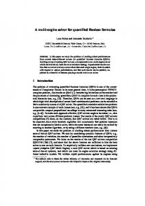
Ranking function synthesis: QuBE & sKizzo vs. Z3

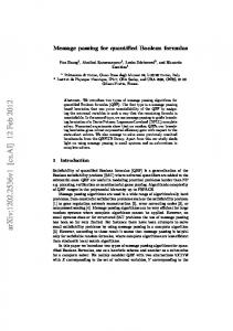
Each universally quantified clause can be independently processed and the resultant formulas/clauses are combined. Another possibility is to apply this approach only to a selected subset of the universally quantified sub-formulas, and rely on the approach described in section IV-D for the remaining ones. Finally, first-order resolution and subsumption can also be used to derive new implied QBV universally quantified clauses and to delete redundant ones. V. E XPERIMENTAL R ESULTS To assess the efficacy of our method we present an evaluation of the performance of a preliminary QBVF solver based on the code-base of the Z3 SMT solver [10]. Our prototype first applies the simplifications described in section IV-A. It then iterates model checking and model finding as described in sections IV-B and IV-C. The benchmarks that we use for our performance comparison are derived from two sources: a) hardware fixpoint checks and b) software ranking function synthesis [8]. It is not trivial to compare our QBVF solver with other systems, since most SMT solvers do not perform well in benchmarks containing bit-vectors and quantifiers. In the past, QBF solvers have been used to attack these problems. We therefore compare to the state-of-the-art QBF solvers sKizzo [3] and QuBE [14]. Formulas in the first set exhibit the structure of fixpoint formulas described in section III. The circuits that we use as benchmarks are derived from a previous evaluation of VCEGAR [18]3 and were extracted using a customized version of the EBMC bounded Model Checker4 , which is able to 3 These

benchmarks are available at http://www.cprover.org/hardware/ is available at http://www.cprover.org/ebmc/

4 EBMC

produce fixpoint checks in QBVF and QBF form. In total, this benchmark set contains 131 files. Our second set of benchmarks cannot be directly encoded in QBF because they contain uninterpreted function symbols. So, we decided to consider only ranking functions that are linear polynomials. By applying this template we can convert the problem to QBF as described in section IV-E. Thus, the problem here is to synthesise the coefficients for the polynomial. Further details, especially on the size of the coefficients, were described previously [8]. All our benchmarks were extracted in two forms: in QBVF form (using SMT-LIB format) and in QBF form (using the QDIMACS format) and they were executed on a Windows HPC cluster of AMD Athlon 2 GHz machines with a time limit of 3600 seconds and a memory limit of 2 GB. As indicated by Figure 2 our approach outperforms the QBF solvers on all instances, sometimes by up to five orders of magnitude and it solves almost all instances in the benchmark set (110 out of 131). Most of the benchmarks solved in this category (87 out of 110) are solved by our simplifications and rewriting rules only. In the remaining cases, the model refinement algorithm takes less then 10 iterations. Figure 3 show the results for the ranking function benchmark set. Again, our algorithm outperforms the QBF solvers by up to five orders of magnitude. The number of iterations required to find a model or prove non-existence of a model in these benchmarks is again very small: almost all instances require only one or two iterations and the maximum number of iterations is 9. Even though our algorithm exhibits similar speedups on both benchmark sets, the behaviour on the second set is quite different: None of the instances in this set is completely solved by the simplifications or rewriting rules. The model finding algorithm is required on each of them.5 VI. R ELATED W ORK In practice it is often the case that uninterpreted functions are not strictly required. In this case, QBVFs can be flattened into either a propositional formula or a quantified Boolean formula (QBF). This is possible because bit-vector variables may be treated as a vector of Boolean variables. Operations on bit-vectors may be bit-blasted, but this approach increases the size of the formula considerably (e.g., quadratically for multipliers), and structural information is lost. In case of quantified formulas, universal quantifiers can be expanded since each is a quantification over a finite domain of values. This usually results in an exponential increase of the formula size and is therefore infeasible in practice. An alternative method is to flatten the QBV formula without expanding the quantifiers. This results in a QBF and off-the-shelf decision procedures (QBF solvers) like sKizzo [3], Quantor [4] or QuBE [14] may be employed to decide the formula. In practice, the performance of QBF solvers has proven to be problematic, however. 5 More

experimental data is provided in Appendix C.

One of the potential issues resulting in bad performance may be the prenex clausal form of QBFs. It has thus been proposed to use non-prenex non-clausal form [11], [15]. This has been demonstrated to be beneficial on certain types of formulas, but all known decision procedures fail to exploit any form of word-level information. A further problem with QBF solvers is that only few of them support certification, especially the construction of models for satisfiable instances. This is an absolute necessity for solvers employed in a synthesis context. SMT QF BV solvers. For some time now, SMT solvers for the quantifier-free fragment of bit-vector logic existed. Usually, those solvers are based on a small set of wordlevel simplifications and subsequent flattening (bit-blasting) to propositional formulas. Some solvers (e.g., SWORD [29]), try to incorporate word-level information while solving the flattened formula. Some tools also have limited support for quantifiers (e.g. BAT [22]), but this is usually restricted to either a single quantifier or a single alternation of quantifiers which may be expanded at feasible cost. Most SMT QF BV solvers support heuristic instantiation of quantifiers based on E-matching [9]. On some unsatisfiable instances, this may terminate with a conclusive result, but it is of course not a solution to the general problem. The method that we propose uses SMT solvers for the quantifier-free fragment to decide intermediate formulas and therefore represents an extension of SMT techniques to the more general QBV logic. Synthesis tools. Finally, there is recent and active interest in using modern SMT solvers in the context of synthesis of inductive loop invariants [25] and synthesis of program fragments [19], such as sorting, matrix multiplication, decompression, graph, and bit-manipulating algorithms. These applications share a common trait in the way they use their underlying symbolic solver. They search a template vocabulary of instructions, that are composed as a model in a satisfying assignment. This approach was the main inspiration for the template based model finder described in section IV-C. VII. C ONCLUSION Quantified bit-vector logic (QBV) is ideally suited as an interface between verification or synthesis tools and underlying decision procedures. Decision procedures for different fragments of this logic are required in virtually every verification or synthesis technique, making QBV one of the most practically relevant logics. We present a new approach to solving quantified bit-vector formulas based on a set of simplifications and rewrite rules, as well as a new model finding algorithm based on an iterative refinement scheme. Through an evaluation on benchmarks that stem from hardware and software applications, we are able to demonstrate that our approach is up to five orders of magnitude faster when compared to a popular approach of flattening the formula to QBF. R EFERENCES [1] C. Barrett, A. Stump, and C. Tinelli, “The Satisfiability Modulo Theories Library (SMT-LIB),” www.SMT-LIB.org, 2010.

[2] C. Barrett and C. Tinelli, “CVC3,” in Proc. of CAV, ser. LNCS, no. 4590. Springer, 2007. [3] M. Benedetti, “Evaluating QBFs via Symbolic Skolemization,” in Proc. of LPAR, ser. LNCS, no. 3452. Springer, 2005. [4] A. Biere, “Resolve and expand,” in Proc. of SAT’04 (Revised Selected Papers), ser. LNCS, no. 3542. Springer, 2005. [5] R. Brummayer and A. Biere, “Boolector: An efficient SMT solver for bit-vectors and arrays,” in Proc. of TACAS, ser. LNCS, no. 5505. Springer, 2009. [6] R. Bruttomesso, A. Cimatti, A. Franz´en, A. Griggio, and R. Sebastiani, “The MathSAT 4 SMT solver,” in CAV, ser. LNCS, no. 5123. Springer, 2008. [7] M. Col´on, “Schema-guided synthesis of imperative programs by constraint solving,” in Proc. of Intl. Symp. on Logic Based Program Synthesis and Transformation, ser. LNCS, no. 3573. Springer, 2005. [8] B. Cook, D. Kroening, P. R¨ummer, and C. M. Wintersteiger, “Ranking function synthesis for bit-vector relations,” in Proc. of TACAS, ser. LNCS, no. 6015. Springer, 2010. [9] L. de Moura and N. Bjørner, “Efficient e-matching for SMT solvers,” in Proc. of CADE, ser. LNCS, no. 4603. Springer, 2007. [10] ——, “Z3: An efficient SMT solver,” in Proc. of TACAS, ser. LNCS, no. 4963. Springer, 2008. [11] U. Egly, M. Seidl, and S. Woltran, “A solver for QBFs in negation normal form,” Constraints, vol. 14, no. 1, 2009. [12] V. Ganesh and D. L. Dill, “A decision procedure for bit-vectors and arrays,” in Proc. of CAV, ser. LNCS, no. 4590. Springer, 2007. [13] Y. Ge and L. de Moura, “Complete instantiation for quantified formulas in satisfiabiliby modulo theories,” in CAV, ser. LNCS, no. 5643. Springer, 2009. [14] E. Giunchiglia, M. Narizzano, and A. Tacchella, “QuBE++: An efficient QBF solver,” in Proc. of FMCAD, ser. LNCS, no. 3312. Springer, 2004. [15] A. Goultiaeva, V. Iverson, and F. Bacchus, “Beyond CNF: A circuitbased QBF solver,” in Proc. of SAT, ser. LNCS, no. 5584. Springer, 2009. [16] S. Gulwani, S. Srivastava, and R. Venkatesan, “Constraint-based invariant inference over predicate abstraction,” in Proc. of VMCAI, ser. LNCS, no. 5403. Springer, 2009. [17] J. Harrison, Handbook of Practical Logic and Automated Reasoning. Cambridge University Press, 2009. [18] H. Jain, D. Kroening, N. Sharygina, and E. M. Clarke, “Word-level predicate-abstraction and refinement techniques for verifying rtl verilog,” IEEE Trans. on CAD of Int. Circuits and Systems, vol. 27, no. 2, 2008. [19] S. Jha, S. Gulwani, S. Seshia, and A. Tiwari, “Oracle-guided componentbased program synthesis,” in Proc. of ICSE. ACM, 2010. [20] B. Jobstmann and R. Bloem, “Optimizations for LTL synthesis,” in FMCAD. IEEE, 2006. [21] D. E. Knuth and P. B. Bendix, “Simple word problems in universal algebra.” in Proc. Conf. on Computational Problems in Abstract Algebra. Pergamon Press, 1970. [22] P. Manolios, S. K. Srinivasan, and D. Vroon, “BAT: The bit-level analysis tool,” in CAV, ser. LNCS, no. 4590. Springer, 2007. [23] A. Pnueli and R. Rosner, “On the synthesis of a reactive module,” in Proc. of POPL. ACM, 1989. [24] A. Podelski and A. Rybalchenko, “A complete method for the synthesis of linear ranking functions,” in Proc. of VMCAI, ser. LNCS, no. 2937. Springer, 2004. [25] S. Srivastava and S. Gulwani, “Program verification using templates over predicate abstraction,” in Proc. of PLDI. ACM, 2009. [26] S. Srivastava, S. Gulwani, and J. S. Foster, “From program verification to program synthesis,” in Proc. of POPL. ACM, 2010. [27] S. Staber and R. Bloem, “Fault localization and correction with QBF,” in SAT, ser. LNCS, no. 4501. Springer, 2007. [28] A. Turing, “Checking a large routine,” in Report of a Conference on High Speed Automatic Calculating Machines, 1949. [29] R. Wille, G. Fey, D. Große, S. Eggersgl¨uß, and R. Drechsler, “Sword: A SAT like prover using word level information,” in Proc. Intl. Conf. on Very Large Scale Integration of System-on-Chip. IEEE, 2007.

A PPENDIX A. Proof of Theorem 1 The proof consists in showing that there is a polynomial reduction from EPR to QBVF and vice-versa. 1) QBVF ⇒ EPR: Given a QBV formula ϕ, w.l.o.g. we assume ϕ is in CNF. The first step is to flat every clause in ϕ. The idea is to avoid nested terms by introducing auxiliary variables. Given a clause ∀x. C[t], where t is a nested term. We convert it into ∀x, y. y 6= t ∨ C[y]. Flattening is applied until all literals in a clause are shallow. For example, the clause ∀x1 , x2 . f (x1 , g(x2 )) ≤ g(x1 ) is reduced to ∀x1 , x2 , y1 , y2 , y3 . y1 6= g(x2 ) ∨ y2 6= f (x1 , y1 ) ∨ y3 6= g(x1 ) ∨ y2 ≤ y3 Next, for each uninterpreted function f where the range is a bit-vector of size n, we create n predicates pf1 , . . . , pfn . Each bit-vector variable and constant is broken into bits. A disequality of the form x 6= f (y) is encoded as ((x1 = ⊤) xor pf1 (y1 , . . . , yn )) ∨ ... ((xm = ⊤) xor pfm (y1 , . . . , yn )) Other atoms are encoded in a similar way. We add two special constants ⊥ and ⊤, add the axiom ⊥ = 6 ⊤, and for each new bit constant c, we add the clause c = ⊥ ∨ c = ⊤. For example, in the following QBV formula, assume all sorts are bit-vectors of size 2. (∀x. f (f (x)) = 0) ∧ f (a) = 2 After flattening, we have:

is equivalent to false. This problem can be avoided by using an approach found in several EPR solvers that do not have support for =. These solvers use the fact that any EPR formula ϕ containing = is equisatisfiable to another EPR formula ϕ′ that does not contain =. The basic idea is to replace = with a new binary predicate isEq, and include the axioms of equality for it. ∀x. isEq(x, x) ∀x, y. ¬isEq(x, y) ∨ isEq(y, x) ∀x, y, z. ¬isEq(x, y) ∨ ¬isEq(y, z) ∨ isEq(x, z) ∀x, y. ¬isEq(x1 , y1 ) ∨ . . . ∨ ¬isEq(xn , yn ) ∨ ¬p(x) ∨ p(y) In fact the last axiom is an axiom scheme, we need one of them for each predicate p in the formula ϕ. B. Proof of Theorem 2 The formula ρ increases monotonically. The conjunct added in every iteration is an instance of φ with all universals replaced by values from the counter-example V , thereby adding new quantifier instances to ρ in every iteration. Since the number of possible instantiations is finite, the process must terminate. In case it terminates with unsat modulo TB, there is no instance of the template TB that satisfies ρ. Since ρ is a conjunction of instances of φ, there is no model for φ modulo TB. C. Experimental results in detail Figures 4, 5, 6 and 7 are bigger versions of the Figures 2 and 3. Tables I and II provide all the runtimes (in seconds) and results of our experiments. They also include the runtimes for the QBF solver Quantor.

(∀x, y. y 6= f (x) ∨ f (y) = 0) ∧ f (a) = 2

[sec] +

Then, after bit-blasting, we have: (∀x1 , x2 , y1 , y2 . ((y1 = ⊤) xor pf1 (x1 , x2 )) ∨ ((y2 = ⊤) xor pf2 (x1 , x2 )) ∨ (¬pf1 (y1 , y2 ) ∧ ¬pf2 (y1 , y2 ))) ∧ ¬pf1 (a1 , a2 ) ∧ pf2 (a1 , a2 ) ∧ (a1 = ⊤ ∨ a1 = ⊥) ∧ (a2 = ⊤ ∨ a2 = ⊥) ∧ ⊤= 6 ⊥ 2) EPR ⇒ QBVF: Any satisfiable EPR formula has a finite Herbrand model. Moreover, a formula containing n constants has a model with a universe of size at most n. Therefore, in principle, it should be straightforward to reduce a EPR formula to QBVF. In principle, we just need to use a bit-vector sort of size ⌈log 2 n⌉. The main problem in this approach is that the EPR formula may contain cardinality constraints such as ∀x. x = a1 ∨ . . . ∨ x = am . For example, this clause is only satisfiable in a model with a universe with size at most m. Now, suppose we have a formula ϕ with n constants and containing a cardinality constraint limiting the universe size to m. If m < ⌈log 2 n⌉, then the QBVF formula ∀x : ⌈log 2 n⌉. x = a1 ∨ . . . ∨ x = am

1k

100

Z3

+ + + + + + + + + +

10 +

1

0.1

0.01 0.01

+ ++ + + + + + + + + + + + + + + + + + + + + + + + + + + + + ++ + + + + + + + + + + ++ + + +++ + + + +++ + ++ + + ++++ ++ 0.1

1

10

100

1k

QuBE

Fig. 4.

Hardware fixpoint checks: QuBE vs. Z3

[sec]

[sec] + 1k

100

Z3

+ + + + + + + + + + ++ ++ + + + ++ + + + + + + + + + + ++ ++ + + + + + + ++ +++ + + + + + +++ ++ + + ++ + + ++ + + ++ + + ++ + + +

10

1

0.1

0.01 0.01

0.1

1

10

100

[sec] +

[sec]

1k

1k

sKizzo

Fig. 5.

+ + 100

Hardware fixpoint checks: sKizzo vs. Z3

+ + + + + + Z3

10

+ +

+

1

+ + + + + + + + + + +

+ +

0.1

+

+

+

[sec] 0.01 0.01

+ 1k

100

Fig. 7.

+ + + + + 10

+ +

1

+ + + + + + + + + + + + + ++

0.1

0.01 0.01

0.1

1

10

100

1k

QuBE

Fig. 6.

Ranking function synthesis: QuBE vs. Z3

1

10

100

1k

sKizzo

+ +

Z3

0.1

[sec]

Ranking function synthesis: sKizzo vs. Z3

[sec]

AR-fixpoint-1.qdimacs AR-fixpoint-10.qdimacs AR-fixpoint-2.qdimacs AR-fixpoint-3.qdimacs AR-fixpoint-4.qdimacs AR-fixpoint-5.qdimacs AR-fixpoint-6.qdimacs AR-fixpoint-7.qdimacs AR-fixpoint-8.qdimacs AR-fixpoint-9.qdimacs cache-coherence-2-fixpoint-1.qdimacs cache-coherence-2-fixpoint-2.qdimacs cache-coherence-2-fixpoint-3.qdimacs cache-coherence-2-fixpoint-4.qdimacs cache-coherence-2-fixpoint-5.qdimacs cache-coherence-2-fixpoint-6.qdimacs cache-coherence-3-fixpoint-1.qdimacs cache-coherence-3-fixpoint-2.qdimacs cache-coherence-3-fixpoint-3.qdimacs ethernet-fixpoint-1.qdimacs ethernet-fixpoint-2.qdimacs ethernet-fixpoint-3.qdimacs ethernet-fixpoint-4.qdimacs itc-b13-fixpoint-1.qdimacs itc-b13-fixpoint-10.qdimacs itc-b13-fixpoint-2.qdimacs itc-b13-fixpoint-3.qdimacs itc-b13-fixpoint-4.qdimacs itc-b13-fixpoint-5.qdimacs itc-b13-fixpoint-6.qdimacs itc-b13-fixpoint-7.qdimacs itc-b13-fixpoint-8.qdimacs itc-b13-fixpoint-9.qdimacs pi-bus-fixpoint-1.qdimacs pi-bus-fixpoint-2.qdimacs pi-bus-fixpoint-3.qdimacs sdlx-fixpoint-1.qdimacs sdlx-fixpoint-10.qdimacs sdlx-fixpoint-2.qdimacs sdlx-fixpoint-3.qdimacs sdlx-fixpoint-4.qdimacs sdlx-fixpoint-5.qdimacs sdlx-fixpoint-6.qdimacs sdlx-fixpoint-7.qdimacs sdlx-fixpoint-8.qdimacs sdlx-fixpoint-9.qdimacs small-bug1-fixpoint-1.qdimacs small-bug1-fixpoint-10.qdimacs small-bug1-fixpoint-2.qdimacs small-bug1-fixpoint-3.qdimacs small-bug1-fixpoint-4.qdimacs small-bug1-fixpoint-5.qdimacs small-bug1-fixpoint-6.qdimacs small-bug1-fixpoint-7.qdimacs small-bug1-fixpoint-8.qdimacs small-bug1-fixpoint-9.qdimacs small-dyn-partition-fixpoint-1.qdimacs small-dyn-partition-fixpoint-10.qdimacs small-dyn-partition-fixpoint-2.qdimacs small-dyn-partition-fixpoint-3.qdimacs small-dyn-partition-fixpoint-4.qdimacs small-dyn-partition-fixpoint-5.qdimacs small-dyn-partition-fixpoint-6.qdimacs small-dyn-partition-fixpoint-7.qdimacs small-dyn-partition-fixpoint-8.qdimacs small-dyn-partition-fixpoint-9.qdimacs

sKizzo TIME MEM TIME TIME MEM MEM MEM MEM MEM MEM 3298.794 TIME TIME TIME MEM TIME TIME TIME TIME 1036.26 MEM MEM TIME 2.277 704.89 5.94 23.183 29.02 850.897 1755.936 277.154 515.197 TIME TIME TIME TIME 3.487 TIME 10.17 298.317 2096.083 490.48 MEM TIME TIME TIME 0.507 1.074 0.48 0.5 0.787 0.873 0.924 0.797 0.96 0.826 0.61 2.206 0.963 0.97 1.064 0.983 1.41 1.123 1.454 2.14

QuBE MEM MEM MEM MEM MEM MEM MEM MEM MEM MEM 193.22 TIME TIME TIME TIME TIME 630.714 TIME TIME 63.214 3266.96 TIME TIME 1.643 105.746 2.483 11.654 14.42 130.657 59.454 41.524 109.94 417.43 TIME TIME TIME 1.61 TIME 2.32 12.854 101.177 202.53 TIME TIME TIME TIME 0.957 0.124 0.08 0.083 0.087 0.097 0.097 0.103 0.107 0.113 0.127 TIME 0.513 4.383 6.043 125.81 776.993 2347.22 2538.42 TIME

Quantor MEM TIME MEM TIME TIME TIME TIME TIME TIME TIME MEM MEM MEM MEM MEM MEM MEM MEM MEM MEM MEM MEM MEM MEM MEM MEM MEM MEM MEM MEM MEM MEM MEM MEM MEM MEM MEM MEM MEM MEM MEM MEM MEM MEM MEM MEM 0.17 0.357 0.147 0.16 0.163 0.19 0.184 0.233 0.21 0.226 0.186 MEM 2.42 4.25 33.11 MEM MEM MEM MEM MEM

Z3 0.077 0.124 0.078 0.078 0.078 0.094 0.109 0.094 0.109 0.109 0.218 1.217 2.417 3.946 7.098 10.748 0.343 2.09 4.461 0.748 2.793 4.696 9.999 0.031 1.357 0.171 0.203 0.328 0.484 0.577 0.764 0.967 1.123 0.437 3.089 5.132 0.124 TIME 0.281 0.608 1.232 2.121 TIME TIME TIME TIME 0 0.094 0.031 0.031 0.046 0.031 0.047 0.062 0.062 0.077 0.015 0.093 0.031 0.016 0.031 0.063 0.046 0.062 0.046 0.078

Result unsat unsat unsat unsat unsat unsat unsat unsat unsat unsat unsat unsat unsat unsat unsat unsat unsat unsat unsat unsat unsat unsat unsat unsat sat unsat sat sat sat sat sat sat sat unsat unsat unsat unsat ? unsat unsat unsat unsat ? ? ? ? sat sat sat sat sat sat sat sat sat sat unsat unsat unsat unsat unsat unsat unsat unsat unsat unsat

small-equiv-fixpoint-1.qdimacs small-equiv-fixpoint-10.qdimacs small-equiv-fixpoint-2.qdimacs small-equiv-fixpoint-3.qdimacs small-equiv-fixpoint-4.qdimacs small-equiv-fixpoint-5.qdimacs small-equiv-fixpoint-6.qdimacs small-equiv-fixpoint-7.qdimacs small-equiv-fixpoint-8.qdimacs small-equiv-fixpoint-9.qdimacs small-pipeline-fixpoint-1.qdimacs small-pipeline-fixpoint-10.qdimacs small-pipeline-fixpoint-2.qdimacs small-pipeline-fixpoint-3.qdimacs small-pipeline-fixpoint-4.qdimacs small-pipeline-fixpoint-5.qdimacs small-pipeline-fixpoint-6.qdimacs small-pipeline-fixpoint-7.qdimacs small-pipeline-fixpoint-8.qdimacs small-pipeline-fixpoint-9.qdimacs small-seq-fixpoint-1.qdimacs small-seq-fixpoint-10.qdimacs small-seq-fixpoint-2.qdimacs small-seq-fixpoint-3.qdimacs small-seq-fixpoint-4.qdimacs small-seq-fixpoint-5.qdimacs small-seq-fixpoint-6.qdimacs small-seq-fixpoint-7.qdimacs small-seq-fixpoint-8.qdimacs small-seq-fixpoint-9.qdimacs small-swap1-fixpoint-1.qdimacs small-swap1-fixpoint-10.qdimacs small-swap1-fixpoint-2.qdimacs small-swap1-fixpoint-3.qdimacs small-swap1-fixpoint-4.qdimacs small-swap1-fixpoint-5.qdimacs small-swap1-fixpoint-6.qdimacs small-swap1-fixpoint-7.qdimacs small-swap1-fixpoint-8.qdimacs small-swap1-fixpoint-9.qdimacs small-swap2-fixpoint-1.qdimacs small-swap2-fixpoint-10.qdimacs small-swap2-fixpoint-2.qdimacs small-swap2-fixpoint-3.qdimacs small-swap2-fixpoint-4.qdimacs small-swap2-fixpoint-5.qdimacs small-swap2-fixpoint-6.qdimacs small-swap2-fixpoint-7.qdimacs small-swap2-fixpoint-8.qdimacs small-swap2-fixpoint-9.qdimacs small-synabs-fixpoint-1.qdimacs small-synabs-fixpoint-10.qdimacs small-synabs-fixpoint-2.qdimacs small-synabs-fixpoint-3.qdimacs small-synabs-fixpoint-4.qdimacs small-synabs-fixpoint-5.qdimacs small-synabs-fixpoint-6.qdimacs small-synabs-fixpoint-7.qdimacs small-synabs-fixpoint-8.qdimacs small-synabs-fixpoint-9.qdimacs usb-phy-fixpoint-1.qdimacs usb-phy-fixpoint-2.qdimacs usb-phy-fixpoint-3.qdimacs usb-phy-fixpoint-4.qdimacs usb-phy-fixpoint-5.qdimacs

TABLE I E XPERIMENTS : H ARDWARE FIXPOINT CHECKS

sKizzo MEM MEM MEM MEM MEM MEM MEM MEM MEM MEM TIME MEM TIME TIME TIME TIME TIME TIME TIME MEM 976.613 TIME MEM MEM TIME TIME TIME TIME TIME TIME 8.813 TIME 24.506 37.483 TIME TIME MEM TIME TIME TIME 0.55 319.853 7.007 38.127 40.767 101.52 81.994 152.68 188.513 318.016 2.2 7.203 1.843 2.273 2.83 3.693 3.887 5.437 7.447 6.907 229.333 TIME TIME TIME TIME

QuBE TIME TIME TIME TIME TIME TIME TIME TIME TIME TIME TIME TIME TIME TIME TIME TIME TIME TIME TIME TIME 3.84 TIME TIME TIME TIME TIME TIME TIME TIME TIME 0.223 2.02 0.36 0.427 0.6 0.79 0.947 1.157 1.383 1.626 0.163 1.787 0.31 0.45 0.543 0.746 0.836 1.11 1.267 1.576 0.197 329.67 0.563 1.806 2.117 4.03 17.686 26.947 61.907 76.893 2.163 50.123 14.86 TIME TIME

Quantor MEM MEM MEM MEM MEM MEM MEM MEM MEM MEM MEM MEM MEM MEM MEM MEM MEM MEM MEM MEM MEM MEM MEM MEM MEM MEM MEM MEM MEM MEM MEM MEM MEM MEM MEM MEM MEM MEM MEM MEM MEM MEM MEM MEM MEM MEM MEM MEM MEM MEM 0.523 MEM MEM MEM MEM MEM MEM MEM MEM MEM MEM MEM MEM MEM MEM

Z3 0.015 TIME TIME TIME TIME TIME TIME TIME TIME TIME 0.016 TIME 0.031 0.093 TIME TIME TIME TIME TIME TIME 0.015 0.031 0.015 0.016 0.015 0.031 0.031 0.031 0.046 0.046 0.015 0.063 0.031 0.016 0.016 0.031 0.031 0.047 0.062 0.062 0 0.047 0.016 0.016 0.016 0.031 0.031 0.046 0.046 0.031 0.016 0.093 0.016 0.016 0.031 0.046 0.047 0.062 0.062 0.078 0.187 1.388 2.496 5.491 7.753

Result sat ? ? ? ? ? ? ? ? ? unsat ? unsat unsat ? ? ? ? ? ? unsat unsat unsat unsat unsat unsat unsat unsat unsat unsat unsat sat sat sat sat sat sat sat sat sat unsat sat unsat sat sat sat sat sat sat sat unsat unsat unsat unsat unsat unsat unsat unsat unsat unsat unsat unsat unsat unsat unsat

1394diag ioctl.c.qdimacs 1394diag isochapi.c.qdimacs audio ac97 common.cpp.qdimacs audio ac97 rtstream.cpp.qdimacs audio ac97 wavepcistream.cpp.qdimacs audio ac97 wavepcistream2.cpp.qdimacs audio ac97 wavepcistream3.cpp.qdimacs audio ddksynth csynth.cpp.qdimacs audio ddksynth csynth2.cpp.qdimacs audio ddksynth voice.cpp.qdimacs audio dmusuart mpu.cpp.qdimacs audio fmsynth miniport.cpp.qdimacs audio fmsynth miniport2.cpp.qdimacs audio gfxswap.xp filter.cpp.qdimacs audio sysfx swap.cpp.qdimacs AVStream hwsim.cpp.qdimacs AVStream image.cpp.qdimacs filesys cdfs allocsup.c.qdimacs filesys cdfs cddata.c.qdimacs filesys cdfs namesup.c.qdimacs filesys cdfs namesup2.c.qdimacs filesys fastfat allocsup.c.qdimacs filesys fastfat cachesup.c.qdimacs filesys fastfat easup.c.qdimacs filesys fastfat write.c.qdimacs filesys filter namelookup.c.qdimacs filesys smbmrx cvsndrcv.c.qdimacs filesys smbmrx midatlas.c.qdimacs filesys smbmrx smbxchng.c.qdimacs general pcidrv sys hw eeprom.c.qdimacs general pcidrv sys hw eeprom2.c.qdimacs general toaster exe notify notify.c.qdimacs hid firefly app firefly.cpp.qdimacs hid hclient ecdisp.c.qdimacs input mouser cseries.c.qdimacs input mouser detect.c.qdimacs input pnpi8042 moudep.c.qdimacs ir smscir io.c.qdimacs kernel agplib init.c.qdimacs kernel agplib intrface.c.qdimacs kernel uagp35 gart.c.qdimacs kmdf AMCC5933 sys S5933DK1.c.qdimacs kmdf osrusbfx2 exe dump.c.qdimacs kmdf osrusbfx2 exe testapp.c.qdimacs kmdf pcidrv sys hw nic init.c.qdimacs kmdf pcidrv sys hw physet.c.qdimacs kmdf usbsamp sys queue.c.qdimacs mmedia gsm610 gsm610.c.qdimacs mmedia gsm610 gsm6102.c.qdimacs mmedia gsm610 gsm6103.c.qdimacs mmedia imaadpcm imaadpcm.c.qdimacs network irda miniport nscirda comm.c.qdimacs network irda miniport nscirda settings.c.qdimacs network ndis coisdn TpiParam.c.qdimacs network ndis e100bex 5x kd mp dbg.c.qdimacs network ndis rtlnwifi extsta st aplst.c.qdimacs network ndis rtlnwifi extsta st misc.c.qdimacs network ndis rtlnwifi hw hw ccmp.c.qdimacs network trans sys notify.c.qdimacs

sKizzo TIME MEM MEM MEM TIME MEM MEM MEM MEM TIME TIME MEM MEM MEM MEM TIME MEM MEM MEM MEM MEM MEM MEM MEM MEM MEM 523.737 40.877 MEM MEM MEM MEM TIME MEM MEM MEM MEM MEM MEM MEM MEM MEM MEM MEM MEM MEM MEM MEM 284.807 371.61 MEM MEM MEM MEM MEM MEM TIME MEM 209.523

QuBE TIME TIME TIME TIME TIME TIME TIME TIME TIME TIME TIME TIME 626.356 TIME TIME TIME TIME TIME TIME TIME TIME TIME TIME TIME TIME TIME TIME TIME TIME TIME TIME TIME TIME TIME TIME 1796.263 TIME TIME TIME TIME TIME TIME TIME TIME TIME TIME TIME TIME TIME TIME TIME TIME TIME TIME TIME TIME TIME TIME TIME

Quantor MEM MEM MEM MEM MEM MEM MEM MEM MEM MEM MEM MEM MEM MEM MEM MEM MEM TIME MEM MEM MEM MEM MEM MEM MEM MEM MEM MEM MEM MEM MEM MEM MEM MEM MEM MEM MEM MEM MEM MEM MEM MEM MEM MEM MEM MEM MEM MEM MEM MEM MEM MEM MEM MEM MEM MEM MEM MEM MEM

Z3 TIME 40.591 0.468 0.202 416.757 0.483 0.219 0.358 0.094 28.08 34.179 0.156 0.109 0.592 TIME TIME 22.401 TIME TIME TIME 0.14 0.187 0.202 6.676 TIME TIME 0.156 0.047 55.816 0.843 0.499 TIME TIME 40.108 0.421 0.031 51.377 TIME 0.109 0.187 40.107 0.141 47.411 TIME 38.016 0.031 TIME 0.187 0.109 0.577 TIME 408.901 515.143 8.158 TIME 42.028 TIME 1.279 6.224

TABLE II E XPERIMENTS : R ANKING FUNCTION SYNTHESIS .

Result ? sat sat sat unsat unsat unsat unsat sat unsat sat sat sat unsat ? ? sat ? ? ? sat sat sat sat ? ? unsat unsat unsat unsat sat ? ? sat sat sat sat ? sat sat sat sat unsat ? sat sat ? sat unsat unsat ? unsat unsat sat ? sat ? sat unsat