Energy-Efficient Spatially-Adaptive Clustering and Routing in Wireless Sensor Networks Hengyu Long∗ Yongpan Liu∗ Xiaoguang Fan∗ Robert P. Dick† Huazhong Yang∗ {ypliu,yanghz}@tsinghua.edu.cn
[email protected] ∗ TNList, EE Dept. † EECS Dept. Tsinghua University University of Michigan Beijing, 100084, China Ann Arbor, MI 48109, U.S.A.
Abstract—Wireless sensor networks hold the potential to open new domains to distributed data acquisition. However, low-cost battery-powered nodes are often used to implement such networks, resulting in tight energy and communication bandwidth constraints. Cluster-based data compression and aggregation helps to reduce communication energy consumption. However, neglecting to adapt cluster sizes to local network conditions has limited the efficiency of previous clustering schemes. We have found that sensor node distances and densities are key factors in clustering. To the best of our knowledge, this is the first work taking these factors into consideration when adaptively forming data aggregation clusters. Compared with previous uniform-size clustering techniques, the proposed algorithm achieves up to 24% communication energy savings in uniform density networks and 36% savings in non-uniform density networks.
I. I NTRODUCTION Wireless Sensor Networks (WSN) are distributed data acquisition systems consisting of numerous wireless sensor nodes. They have the potential to allow sensing in applications and environments where it was previously impossible or prohibitively expensive. For example, WSNs may be used in weather monitoring, security, tactical surveillance, disaster management, and intelligent traffic control applications [1]. Infrastructure-free operation and low node costs are the source of much of their benefit. However, these beneficial attributes exact a penalty. Distributed infrastructure-free operation in remote locations makes replacing batteries expensive. Energy constraints are therefore extremely tight. Tight energy constraints combined with the requirement for low node cost limit wireless communication bandwidth. Data compression and aggregation have the potential to improve WSN energy efficiency and minimize communication. Researchers have previously considered data aggregation and compression in WSNs. We divide existed strategies into two categories. In single-input coding [2], [3] each node can consider data from only one other source during data compression. In multi-input coding strategies [4], [5], [6], [7], [8], aggregation exploits correlation in data from multiple sources. Multi-input coding strategies are generally based on clusters of WSN nodes. We therefore call them cluster compression. Cluster-based routing schemes perform data aggregation only in cluster-heads, while in singe-input routing schemes every intermediate node performs data aggregation. This property generally reduces the communication and computation costs of cluster compression, relative to single-input compression: cluster compression generally scales better. This paper focuses on cluster compression. This work was supported in part by the 863 Program under award 2006AA01Z224, in part by the NSFC under awards 90207001 and 60871005, and in part by NSF under awards CNS-0347941 and CNS-0721978.
There is a large body of work [9], [10] on clustering and aggregating schemes for WSNs. Past work mainly focused on maintaining network connectivity but neglected setting cluster sizes to minimize energy consumption. Marco et al. investigated the capability of large-scale sensor networks to gather and communicate a two-dimension data field and presented theoretical limits on data compression [11]. Heinzelman, Chandrakasan, and Balakrishnan proposed the lowenergy adaptive clustering hierarchical (LEACH) method [6], in which clusters are formed by selecting a specific number of sensor nodes as cluster heads. Nodes are placed in clusters to minimize their individual communication energy consumptions. PEGASIS [12] is an extension of LEACH, in which all nodes are organized into a chain and each node transmits data only to its neighbor. However, neither LEACH nor PEGASIS optimize cluster sizes to minimize energy consumptions considering spatial correlation. Recently, Pattem, Krishnamachari, and Govindan [13] presented a uniform-size clustering approach for WSNs based on joint entropy analysis. This work shows the impact of spatial correlation on data aggregation. Experimental results showed that static uniform clustering can provide near-optimal performance for a wide range of spatial correlations. However, their approach is limited to uniform-size clusters. Soro and Heinzelman first introduced the non-uniform clustering [14]. By assuming that the cluster-heads have predetermined locations, the proposed approach divides the sensor nodes into circular-organized layers, and gains the network a longer lifetime. Recently, Jin et al. introduced a non-uniform ring-shaped clustering scheme and optimized the thickness of each ring [15]. However, these projects [14], [15] rely on the regular geometrical-shaped clusters and the assumption that heterogeneous sensor nodes are used. These assumptions do not hold for some applications. To the best of our knowledge, this is the first article to present a spatially-adaptive clustering scheme for WSNs without any geometry restrictions. Spatial correlation factors, such as node-to-sink distance and sensor density, are used to adapt cluster size depending on data correlation and spatial properties to minimize routing energy. This work makes the following contributions. (1) We present a set of system models, including network model, data aggregation model, and data transmission model to estimate the energy costs of clustering and data collecting in WSNs. (2) Given sensor density and node-to-sink distance, we are the first to present an analytical method of determining optimal aggregation cluster size. We find that optimal cluster size increases with the distance to the network sink node and with increasing sensor density. Compared with a uniform cluster size approach, we show that adaptive cluster sizes always improve energy savings for both
4
x 10
total transmission cost inter−cluster cost intra−cluster cost
total transmis sion cost (µJ)
12 10
d0
network size = 20 × 20 d0=15, c=40
8
Sink 6
optimal cluster size
4
di
d
2 0
2
4
6
8
10
12
14
16
cluster size
Fig. 3. Fig. 1.
Fig. 2.
Random graph.
Intra-cluster and inter-cluster costs.
Distance and density based clustering features.
uniform (up to 24%) and nonuniform (up to 36%) density WSNs. The impacts of factors such as sink position, network size, density, and data correlation on the proposed technique are determined. II. M OTIVATION This section provides the motivation of the proposed spatial adaptive clustering and routing scheme. We first discuss the relationship between the intra-cluster and inter-cluster cost. We then summarize the basic idea behind distance- and densityadaptive clustering. II.A. Intra- and Inter-Cluster Costs The total cluster communication energy is composed of two parts. The intra-cluster cost is the energy consumed by all data communication from the member nodes in the cluster to the cluster-head, which is a special node to aggregate data from other nodes in a cluster. The inter-cluster cost is the energy consumed by communication between the cluster-head and the sink node. Intra- and inter-cluster costs are functions of cluster size. If the entire WSN is composed of one large cluster, there is no inter-cluster cost but the intra-cluster cost is extremely high. At the other extreme, each cluster contains only a single node, for which the inter-cluster cost is high but the intra-cluster cost is low. Figure 1 shows how the intraand inter-cluster costs vary as a function of cluster size (we will give details on the setup below). The total cost function is convex. Our goal is to find the optimal cluster size. II.B. Distance and Density Based Clustering (DDC) Our idea is to take distance and density into consideration to form an adaptive clustering scheme. As Figure 2(a) shows, if the distance of a region from the sink is large, the optimal cluster size is also large because any data transmitted from this point must be repeatedly retransmitted before reaching the sink. The converse is true for clusters near the sink node: smaller clusters are better in this case. Figure 2(b) compares regions with different densities. In dense regions, large clusters are better because high spatial data correlation leads to a good compression ratio. In summary, distance and density are two key factors in clustering. Based on this observation, we develop our network model.
III. F ORMULATION This section describes the modeling methodologies used in our analysis and experiments. We first describe the network model including sensor nodes, wireless communication, and statistical data properties. Second, we propose a common data aggregation model to estimate the performance of multi-input compression algorithms in each cluster. Third, we present energy models for wireless communication and provide typical values for the parameters. Finally, we explain our method of computing total data gathering energy consumption for both inter-cluster and intra-cluster cases. III.A. Sensor Network Model We aim to build a network model of WSNs that supports applications with a wide range of characteristics. A connected graph G = (V, E) is used to describe the network. Each vertex vi ∈ V represents a sensor node. Each edge ei ∈ E is an available wireless communication link. The data gathering tree T = (V, ET ) is defined as a subgraph of G. The tree indicates the communication paths from every source to the sink node. Each node is assumed to generate the same amount of data b per cycle. For each edge ei in T , the flow amount is denoted as the number of bits bi that transports over ei . Example network instances can be generated in MATLAB as shown in Figure 3. Sensor nodes in our model have a uniform coarse-grained distribution and a uniform random fine-grained distribution. To generate an n × n node network of this type, we first partition the region into (n − ) × (n − ) square elements, each of which has a side length of d . The n sensor nodes are located near the n grid vertices, offset by random two-dimensional offsets drj , which are constrained as follows: −d / < drj < d /. Each node is linked to its neighbors directly and di is the Euclidean distance along the ith edge. Figure 3 shows a × random graph generated by this method. III.B. Data Aggregation Model Data correlation exists in many applications. Several approaches have been proposed to model the correlation, e.g., the entropy-based model [13] and the inverse proportional model [2]. However, real compression algorithms and data from real applications have not been used in their models. In order to draw a more accurate and realistic data aggregation model, we use data from the Tropical Atmosphere Ocean (TAO) project [16], on which the differential coding compression algorithm [17] is used. TAO provides collections of oceanographic and surface meteorological data sets from moored ocean buoys. It consists of records including air temperature, sea level pressure, and sea surface temperature. We use the data set of sea surface temperature because the observed points are not far from each other (depth from 1 m
TABLE II T YPICAL T RANSMISSION PARAMETER VALUES FOR µAMPS-1 9
max error rate = 6.32%
aggregation level (b 0 bis)
8
s=9
7
Parameter Value
actual data approximations
s=8
α 2.018 µJ
β 1.0 µJ
η 3.5
s=7 6
s=6 5
s=5
4
s=4
3
s=3
2
when s = 2, c = 40 Bs(d0)=b 0+(s−1)(1−e−d0/(c+s)⋅ ln2)b 0
b01 0
0
100
200
300
400
500
source distance (m)
Fig. 4.
Compression fitting model.
TABLE I F ITTING PARAMETER VARIATION Cluster Size Most Fitting c
2 40
3 41
4 42
5 42
6 43
7 45
8 47
9 48
to 500 m), and exhibit spatial data correlation. To compare the number of bits before and after compression, we do differential encoding as follows. The sources in a cluster are coded along aggregation tree paths from the cluster head to the farthest node in order. When data are encoded within a cluster, we chose the nearest neighbor to be its differential coding reference. Based on the compression algorithm and data sets, we compress data from clusters to show the relationship between real compressed data size and their inter-node distance d in Figure 4. We show results for cluster size s ranging from 2 to 9. An analytical expression is needed to model the curve. Pattem et al. [13] presented the following formula to model the average joint entropy of an s-node cluster: Ã ! Bs (d ) = b + (s − ) − d b (1) c + where b is the number of bits generated by each source, c is a constant characterizing the spatial data correlation, and Bs (d ) is the number of compressed bits generated by the cluster-head in an s-node cluster with inter-node distance d . Bs (d ) is chosen such that when c = d , data from the second source can be compressed to half their initial size. In the sea surface temperature data set, the best c is 40. Experiments show that Equation 1 has an average error of 5.4% and maximum error of 18.5%. We will further reduce the modeling error based on the following observations: (1) the empirical curve in Figure 4 suggests an exponential trend and (2) as Table I has shown, the optimal c value increases with cluster size. Therefore, we propose the following improved model: ³ ´ − d ln Bs (d ) = b + (s − ) − e cinit +s b (2) where cinit is the initial optimal value for the minimal cluster. Other parameters have the same meanings as in Equation 1. The fitting curves of Equation 2 are shown in Figure 4. Experiments show that the proposed model has 2.63% error on average and a maximum error 6.32%. We consider this accurate enough for use in system-level analysis. Thus, we have a closed-form expression for quantifying correlation. This is a general way to characterize the spatial correlation in a specific application data set.
III.C. Data Transmission Model Node-to-node wireless communication includes transmitting and receiving phases. Let pi be the total bits transmitted along edge ei . Min and Chandrakasan [18] models the energy consumption of node-to-node communication as follows: (3) E(di ) = pi · (α + βdηi ) where di is the transmission distance on edge ei and η is the path loss exponent. α and β are constants indicating the distance-independent and distance-dependent energy components for one-bit communication. µAMPS-1 is a hardware platform for distributed microsensor networks using commercial components. Based on measured parameters [18], we report typical values of α, β, and η for the µAMPS-1 platform in Table II. This model can be easily extended to other platforms by changing the values of its parameters. III.D. Total Data Gathering Cost In cluster-based data gathering, each cluster’s communication costs can be divided into intra-cluster and inter-cluster costs. We denote the intra-cluster cost as Cintra,k . A tree Tk is used to collect data from cluster k. According to Equation 3, Cintra,k is calculated as follows: X X Cintra,k = E(di ) = pi · (α + βdηi ) (4) ei ∈Tk
ei ∈Tk
where di is the transmission distance on the edge ei , and pi is the number of bits transmitted on ei . The inter-cluster cost Cinter,k of cluster k is defined as the energy consumed by transmitting compressed data from the cluster-head to the sink via route Rk . Equation 2 can be used to estimate the size of compressed data Bsk in an s-node cluster k. Therefore, we can calculate Cinter,k based on Equation 3. X X Cinter,k = E(di ) = Bsk · (α + βdηi ) (5) ei ∈Rk
ei ∈Rk
Finally, we get P the total transmission cost of the network Cnetwork = k (Cintra,k + Cinter,k ) by summing all the cluster’s communication costs. IV. P ROPOSED DDC A PPROACH As explained in Section II, distance and density should be considered in clustering for data aggregation and compression. This section describes DDC, an adaptive clustering algorithm that balances the intra-cluster and inter-cluster cost by locally tuning cluster size. We first give an analytical framework for determining energy-efficient cluster size. Based on this analysis, we present the DDC spatially-adaptive clustering and routing algorithm. IV.A. Determine DDC Size We now present a theoretical framework to determine energy-optimal data gathering cluster sizes, considering distance and density. Suppose m sensor nodes are deployed near vertices of a mesh network (see Figure 3) with an average nearest-neighbor distance of d . Each sensor generates b bits of data per cycle. As Figure 5(a) shows, the distance between the sink and this region is d. We divide all sensor nodes into m /s s-node clusters. For each cluster, the sensor node nearest to the sink is designated as the cluster-head. After the
Fig. 5. Determine the optimal cluster size considering distance and density.
cluster-head completes data aggregation, the compressed data are sent to the sink. Therefore, the problem can be formulated as follows. Given a sensor network structure, determine the optimal cluster size(s) to minimize the total energy cost of transmitting data from this region to the sink. According to the models presented in Section III, we now derive the energy cost expressions for intra-cluster and intercluster components and determine the optimal number of nodes in the cluster sopt√. We first calculate the intra-cluster component of the cost. s nodes are along the side of each s-node square cluster (see Figure 5(b)). Observe that the intracluster energy cost Cintra,k is the sum of communication energies of sensor nodes in cluster k. We denote the number of retransmissions a sensor node i requires to transmit a packet to its cluster head as λi . To simplify analysis, we assume each hop communication distance is equal to the average distance d shown in Figure 3. Manhattan distance is used to estimate the communication routing path and hop number from each node to sink. Both approximations are reasonably accurate due to regular network structure defined in Figure 3. It can also be used for non-regular structure, if the whole network can be divided into nearly regular regions. The value of this model is also supported by experimental evidence of energy savings resulting from cluster sizing based on the Equation 6 (see Section V), where both approximations are relaxed. Thus, the intra-cluster cost for cluster k follows. λi s X s X X η (α + βdj ) ≈ b Cintra,k = b λi (α + βdη ) i= j=
i=
√ ≈ b s( s − )(α + βdη ) (6) where dj is the one-hop communication distance. We now consider inter-cluster communication energy. Suppose the distance d between the sink and a region is much greater than the diameter of the region. We can approximate the distance between each cluster-head to sink in this region as d. For a connected regular sensor network, other sensor nodes serve as relay stations between this region and the sink. The node-to-node distance is d . Therefore, dd hops are required to reach the sink node. Based on Equation 2, the inter-cluster cost for cluster k is calculated as follows: d d Cinter,k = b (( − e− c+s ln )(s − ) + ) (α + βdη ) (7) d The total cost of the m /s clusters in this region is obtained as follows: X Cwsn = (Cintra,k + Cinter,k ) √ = b [s( s − )(α + βdη ) + d
(( − e− c+s ln )(s − ) + ) × m d/d (α + βdη )] s
(8)
By setting the derivative to zero, the optimal value of cluster size sopt can be obtained. Considering that the cluster size s is much less than c, we simplify the expression by ignoring s in the exponential term and achieve an analytical result for the optimal cluster size. sµ ¶ d − d ln sopt = (9) e c d Equation 9 can be used to determine the optimal cluster size sopt of a region with specific distance and density. Further views on Equation 9 reveal the relationship between the optimal cluster size sopt and spatial correlation parameters, such as d and c. If the node-to-sink distance d is long or the correlation level c is high, large clusters are better than smaller ones. The optimal cluster size sopt , however, is inversely proportional to d . This implies that sopt is larger in dense regions (small d ) and smaller in sparse regions (large d ). This fits well with the analysis in Section II. IV.B. DDC Algorithm Equation 9 provides a way to determine the optimal cluster size, and served to guide our design of the DDC algorithm (see Algorithm 1). The clustering flow can be divided into three steps: (1) select a region for clustering; (2) decide the optimal cluster size for a region; (3) form the cluster by absorbing other nodes; and repeat the process. Lines 1–2 initialize the clustering progress. Lines 3–18 show the iterative clustering procedure. We start clustering in the regions farthest from the sink. At the beginning of each clustering progress, the farthest unclustered node from sink is selected as the first node in the cluster (Line 5). We use its distance d to the sink as the reference to calculate the optimal cluster size (Line 6). The cluster’s nearest unclustered neighbor nodes are absorbed as members in the cluster (Line 8–14). Once the optimal cluster size sopt is reached, the process is terminated and another clustering process starts, until all nodes belong to clusters (Line 15–18). Line 19 chooses a proper cluster-head for each cluster based on the shortest distance metric. Algorithm 1 DDC Algorithm 1: 2: 3: 4: 5: 6: 7: 8: 9: 10: 11: 12: 13: 14: 15: 16: 17: 18: 19:
insert all nodes into aggregate S aggregate CS (cluster set) = null (empty set) while S 6= null do aggregate CC (current cluster) = null find the farthest node from the sink in S : vi calculate the optimal cluster size : sopt insert vi into CC while S 6= null do if size of CC scc = sopt then break end if find neighbors of CC in S : nb find a node vn in nb to minimize the cluster’s width and height insert vn into CC end while insert CC into CS remove nodes in CC from S end while select the nearest-to-sink node as the cluster-head for each cluster
V. E XPERIMENTAL R ESULTS This section first describes the experimental setup. We then compare the proposed DDC algorithm with a uniform-size clustering method. Both uniform density and non-uniform density networks are considered.
o sink
network size = 20 × 20
o
sensor
intra−cluster route
18
energy saving percentage
17
o
15.59% saving
α = 2.018µJ β=1.0µJ η=3.5
16 15
d =10 0
d0=20
14
d0=40
13 12 11 10 9 8
network size = 20 × 20
o 0
sink position = (1,1)
sink position = (10,10)
Fig. 6.
2
10
10
correlation level : c
Fig. 8.
DDC’s adaptivity.
1
10
Impact of correlation level on DDC energy savings.
5
x 10
35
transmission cost (µJ)
2.5
2
1.5
c=40 α=2.018µJ β=1.0µJ η=3.5
0.5
0 10
12
14
16
18
20
22
24
26
28
α begins to predominate
30
19.67% saving
d0=15 1
α = 0.1 µJ α = 2 µJ α = 10 µJ
network size = 20 × 20
24.01% saving sink position = (1,1) , DDC sink position = (1,1) , Uniform sink position = (n/2,n/2), DDC sink position = (n/2,n/2), Uniform sink position = (n/3,n/3), DDC sink position = (n/3,n/3), Uniform
energy saving percentage
3
25 20
α has no effects when β is high
15
the effects of β decline
10
β ’s typical range
d0=15, c=40
5
η=3.5 30
0 −14 10
Fig. 7. DDC vs uniform size clustering in different network sizes and with different sink positions.
V.A. Experimental Setup We choose the total transmission cost per cycle to analyze the performance of DDC and to compare it to the uniform square clustering scheme, which divides the network into uniform-size clusters. The networks in the experiments are randomly generated by the method presented in Section III-A. We vary the parameters of the model in ranges that might be encountered in a WSN and examine the impact on the total cost. The following experimental parameters are used: • Network size: 10×10–30×30 nodes. • Node-to-node distance d : 10 m–40 m. • Data correlation constant c: 1–100. • Distance-independent energy constant α: 0.1 µJ–10 µJ • Distance-dependent energy constant β: 0.01 µJ–2.0 µJ V.B. DDC in Uniform Density Network Figure 6 illustrates spatially-adaptive clustering using the DDC algorithm. Note the variation in cluster size with changing distance to the sink. Figure 7 compares the energy cost of DDC with uniform-size clustering for different network size. The transmission energy saved by DDC increases with network size. The spatially-adaptive strategy achieves more savings due to greater optimal cluster size differences in larger networks. When the network size reach 30×30 nodes, the total energy savings are up to 24%. Figure 7 also shows the energy savings achieved by the DDC approach for different sink node locations. However, the absolute energy cost may vary, which implies that energy can be reduced by carefully selecting the different sink node’s location. These results indicate that the proposed DDC approach is more energy efficient than uniform-size clustering for a wide range of network sizes. Compared with uniform-size clustering, Figure 8 shows the variation of energy savings by DDC for different densities d and correlation levels c in a 20×20 network. The energy
−12
10
−10
−8
10
10
−6
10
β
network size n × n
Fig. 9.
Impact of α and β on DDC energy savings.
savings due to DDC increase with network density. Increased node density has the same effects as bigger network size. Figure 8 also indicates that for very high or low correlation levels c, the advantage of DDC wanes. This can be intuitively explained by the following extreme case. When the correlation level is high enough to make the best cluster size equal to the network size, DDC has no advantage over uniform-size clustering. When the correlation level is very low, clustering does not help. Therefore, DDC shows a more distinct advantage in dense networks than in sparse networks. With a typical correlation level c, DDC has a considerable energy saving (up to 16% for a 20×20 network), but when c is too low or too high, the advantage of DDC decreases. Figure 9 shows the impacts of distance-dependent and distance-independent communication energy costs on the energy saving of DDC compared with uniform-size clustering. β varies on the (logarithmic) x-axis of Figure 9. Each curve is drawn with a distinct α, ranging from 0.1 µJ to 10 µJ. In the typical ranges for β (0.001 µJ to 1 µJ) and α, DDC has a distinct advantage over uniform-size clustering (more than 20% energy savings). The energy savings reduce when β increases over a threshold, because larger β leads to more sensitivity to the transmission distance. When both β and α are small (α = . µJ), the transmission cost approaches zero. Thus, the difference between DDC and uniform clustering decreases. However, when α is larger, DDC remains superior. V.C. DDC in Non-Uniform Density Domain In order to monitor different physical phenomenon, sensor networks with non-uniform densities can be deployed. In this section, we evaluate DDC’s advantages in networks composed of two regions of differing densities. For general networks with non-uniform density, density-based partitioning should be done before clustering. However, a detailed treatment of the partitioning problem is beyond the scope of this paper.
40
d0=16 in part A
Fig. 10. Density variation and area variation in non-uniform density domain.
energy saving percentage
35.85% saving
d0=8 in part A
30
25
approximatly SA= SB
20
0
energy saving percentage
32
0.1
d0=15 in part A, c=40
30
0.2
0.3
0.4
0.5
0.6
0.7
0.8
0.9
1
area ratio SB/(SA+SB)
sensing area = 15 × 15 m2
30.61% evergy saving
d0=12 in part A
35
Fig. 12.
Area ratio impact on DDC energy savings.
28 26 24
density−uniform situation
22 0.2 0.2
0.4
0.6
0.8
1
1.2
1.4
1.6
1.8
2
density ratio
Fig. 11.
Density ratio impact on DDC energy savings.
This section compares DDC’s energy cost of data gathering with that of the uniform size clustering scheme for two-part non-uniform density domains shown in Figure 10(a). Figure 11 shows the variation in DDC energy savings, relative to uniform-size clustering, when the density of part B is changed from half to double the value in part A. We observe a rapid decrease in energy savings when the density approaches 1. This corresponds to the uniform-density case. From the curve shape we draw the conclusion that DDC saves more energy in non-uniform density networks. Suppose the densities of Region A and B in Figure 10(b) are fixed, and the area of Region B increases from zero to the whole sensing field. Figure 12 shows the DDC energy savings trend when the area ratio between Region A and B changes. We observe that energy savings reduce at the high and low area ratios in Figure 12, because those situations approximate the uniform-density case. We can also observe that the energy saved by DDC increases (up to 36%) in the middle segments of the curves. It can be explained by the fact that the area variation of Region B makes Region A a shapeirregular field, for which the uniform-size clustering scheme is poorly suited. In contrast, DDC algorithm does not have such a limit. This analysis demonstrates that DDC has the most benefit over uniform clustering in energy consumption for non-uniform density sensor fields. VI. C ONCLUSIONS Distance and density are two key factors in WSN data aggregation and clustering techniques. We have shown how these two factors impact energy consumption, and have proposed DDC, an energy-efficient adaptive-size cluster formation algorithm that considers the impact of these factors. Experimental results show that DDC performs well in uniform and nonuniform density networks and improves energy consumption up to 24% and 36% relative to past work. R EFERENCES [1] C. Y. Chong and S. P. Kumar, “Sensor networks: evolution, opportunities, and challenges,” Proc. of the IEEE, vol. 91, pp. 1247–1256, 2003.
[2] P. V. Rickenbach and R. Wattenhofer, “Gathering correlated data in sensor networks,” in Proc. Joint Wkshp. Foundations of Mobile Computing, Oct. 2004, pp. 60–66. [3] R. Cristescu, B. Beferull-Lozano, and M. Vetterli, “Networked Slepian-Wolf: theory, algorithms, and scaling laws,” IEEE Trans. Information Theory, vol. 51, pp. 4057–4073, Dec. 2005. [4] A. Goel and D. Estrin, “Simultaneous optimization for concave costs: Single sink aggregation or single source buy-at-bulk,” Algorithmica, vol. 43, pp. 5–15, Jan. 2005. [5] Y. Yu, B. Krishnamachari, and V. K. Prasanna, “Energy-latency tradeoffs for data gathering in wireless sensor networks,” in Proc. Int. Conf. Computer Communications, Mar. 2004, pp. 244– 255. [6] W. R. Heinzelman, A. Chandrakasan, and H. Balakrishnan, “Energy-efficient communication protocol for wireless microsensor networks,” in Proc. Hawaii Int. Conf. on System Sciences, Jan. 2000, pp. 3005–3014. [7] O. Younis and S. Fahmy, “Distributed clustering in ad-hoc sensor networks: A hybrid, energy-efficient approach,” in Proc. Int. Conf. Computer Communications, Mar. 2004, pp. 629–640. [8] F. Ye, G. Zhong, J. Cheng, S. Lu, and L. Zhang, “PEAS: A robust energy conserving protocol for long-lived sensor networks,” in Proc. Int. Conf. Distributed Computing Systems, Jan. 2003, pp. 28–37. [9] D. Baker and A. Ephremides, “The Architectural Organization of a Mobile Radio Network via a Distributed Algorithm,” IEEE Trans. Communications, vol. 29, no. 11, pp. 1694–1701, Nov. 1981. [10] A. D. Amis, R. Prakash, T. H. P. Vuong, and D. T. Huynh, “Max-min d-cluster formation in wireless ad hoc networks,” in Proc. Int. Conf. Computer Communications, Mar. 2000, pp. 32– 41. [11] D. Marco, E. J. Duarte-Melo, M. Liu, and D. L. Neuhoff, “On the many-to-one transport capacity of a dense wireless sensor network and the compressibility of its data,” Lecture Notes on Computer Science, pp. 1–16, Oct. 2003. [12] S. Lindsey and C. S. Raghavendra, “PEGASIS: Power-efficient gathering in sensor information systems,” in Proc. Aerospace Conf., vol. 3, Apr. 2002, pp. 1125–1130. [13] S. Pattem, B. Krishnamachari, and R. Govindan, “The impact of spatial correlation on routing with compression in wireless sensor networks,” in Proc. Int. Symp. Information Processing in Sensor Networks, Apr. 2004, pp. 28–35. [14] S. Soro and W. R. Heinzelman, “Prolonging the lifetime of wireless sensor networks via unequal clustering,” in Proc. Int. Parallel and Distributed Processing Symp., Apr. 2005, pp. 236– 240. [15] Y. Jin, L. Wang, Y. Kim, and X. Yang, “Energy efficient nonuniform clustering division scheme in wireless sensor networks,” Wireless Personal Communication, vol. 45, pp. 31–43, Aug. 2008. [16] “Tropical atmosphere ocean project,” http://www.pmel.noaa. gov/tao/. [17] A. P. Clark, Principles of digital data transmision. London, Pentech Press, 1983. [18] R. Min and A. Chandrakasan, “A framework for energy-scalable communication in high-density wireless networks,” in Proc. Int. Symp. Low Power Electronics & Design, Aug. 2002, pp. 36–41.