Ensemble Deep Learning for Biomedical Time Series Classification

Hindawi Publishing Corporation Computational Intelligence and Neuroscience Volume 2016, Article ID 6212684, 13 pages http://dx.doi.org/10.1155/2016/6212684

Research Article Ensemble Deep Learning for Biomedical Time Series Classification Lin-peng Jin1,2 and Jun Dong1 1

Suzhou Institute of Nanotech and Nanobionics, Chinese Academy of Sciences, Suzhou 215123, China University of Chinese Academy of Sciences, Beijing 100049, China

2

Correspondence should be addressed to Jun Dong; [email protected] Received 12 January 2016; Revised 10 April 2016; Accepted 4 May 2016 Academic Editor: Leonardo Franco Copyright © 2016 L.-p. Jin and J. Dong. This is an open access article distributed under the Creative Commons Attribution License, which permits unrestricted use, distribution, and reproduction in any medium, provided the original work is properly cited. Ensemble learning has been proved to improve the generalization ability effectively in both theory and practice. In this paper, we briefly outline the current status of research on it first. Then, a new deep neural network-based ensemble method that integrates filtering views, local views, distorted views, explicit training, implicit training, subview prediction, and Simple Average is proposed for biomedical time series classification. Finally, we validate its effectiveness on the Chinese Cardiovascular Disease Database containing a large number of electrocardiogram recordings. The experimental results show that the proposed method has certain advantages compared to some well-known ensemble methods, such as Bagging and AdaBoost.

1. Introduction In the field of pattern recognition, the target of classification is to construct a decision-making function in nature. We can obtain the best ones via simple calculation for linear classification problems, while it is not easy to determine the best ones for nonlinear classification problems, such as image recognition and biomedical time series classification. The processing flow of traditional methods is such that feature vectors are extracted from raw data first (feature selection is conducted when necessary), and then a suitable model based on them is employed for classification. If we let 𝑓(𝑥) and 𝑔(𝑥) be the corresponding function of these two parts, the constructed decision-making function can be written as 𝑔(𝑓(𝑥)). However, with many of the existing feature extraction technologies and classification algorithms, we cannot have highly complicated nonlinear functions. For example, principal component analysis and independent component analysis are both linear dimensionality reduction algorithms, the wavelet transformation is a simple integral transformation, and the Gaussian mixture model is made of a finite number of Gaussian functions. Therefore, many traditional methods do not perform very well in hard artificial intelligence task.

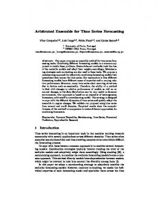
Achieving great success in complicated fields of pattern recognition in recent years, deep learning [1, 2] is a deep neural network (DNN) with more than 3 layers, which inherently fuses “feature extraction” and “classification” into a signal learning body and directly constructs a decisionmaking function. Obviously, its ability to construct nonlinear functions becomes strong with the increasing number of layers and neurons, but the number of network weights that need to be adjusted is significantly increased. On the other hand, with ensemble learning that combines multiple classifiers [3], we can also have complicated decision-making functions. As shown in Figure 1, we can obtain a nonlinear classification model via seven linear classifiers (the filled and unfilled regions denote two classes, resp.). In fact, the constructive mechanism of ensemble learning is the same as that of support vector machine, which constructs nonlinear functions by combining multiple kernel functions. The pioneering work of ensemble learning was done in 1990 [4, 5], which proved that multiple weak learning algorithms could be converted into a strong learning algorithm in theory, and since then many scholars have carried out widespread and thorough research. In general, ensemblelearning algorithms consist of two parts: how to generate differentiated individual classifiers and how to fuse them,

2

Computational Intelligence and Neuroscience

+1 −1

−1

Figure 1: Ensemble learning.

namely, generation strategies and fusion strategies. Next, we will provide a brief review of both of them. There are two kinds of generation strategies, namely, the heterogeneous type and the homogeneous type. The former is such that individual classifiers are generated using different learning algorithms. We will not elaborate on this type since it is relatively simple. The latter uses the same learning algorithm, so different settings (such as learning parameters and training samples) are necessary. Many methods have been developed for this subject and can be divided into four categories. The first way is to manipulate training samples. For instance, Bagging [7] creates multiple data sets by sampling with replacement from the original training samples, each of which is used to train an individual classifier. Boosting [8–10] is another example, in which the learning algorithm uses a different weighting or distribution over the training samples at each iteration, according to the errors of the individual classifiers. There are also other approaches, such as CrossValidated Committees [11], Wagging [12], and Arcing [13]. The second way is to manipulate input features. Random Subspace [14] generates different randomly selected subsets of input features and trains an individual classifier on each of them, while Input Decimation [15] trains the individual classifier only on the most correlated subset of input features for each class. There are also other methods, such as Rotation Forest [16] and Similarity-Based Feature Space [17]. The third way is to manipulate class labels. For instance, Output Coding [18–20] decomposes a multiclassification task into a series of binary-classification subtasks and trains individual classifiers for them. Class-Switching [21, 22] is another example, which generates an individual classifier based on randomly changing the class label of a fraction of the training samples. The last way is to inject randomness into the learning algorithm. For example, using the backpropagation (BP) algorithm, the resulting classifiers can be quite different if neural networks with different initial weights are applied to the same training samples [23]. There are also other approaches such as Randomized First-Order Inductive Learner [24] and Random Forest [25]. In a word, the core of generation strategies is to make individual classifiers different (independent errors and diversity), and only when this condition is satisfied can the classification performance be improved; that is, a good decision-making function can be constructed. As for fusion strategies, Major Voting [26] is one of the most popular methods, in which each individual classifier votes for a specific class, and the predicted class is the one that collects

the largest number of votes. Simple Average and Weighted Average [27] are also commonly used. Besides them, one can also employ other methods to combining individual classifiers, such as Dempster-Shafer Combination Rules [28], Stacking Method [29], and Second-Level Trainable Combiners [30]. Since both deep learning and ensemble learning have advantages in constructing complicated nonlinear functions, the combination of the two can better handle hard artificial intelligence tasks. Deng and Platt [31] adopted linear and log-linear stacking methods to fuse convolutional, recurrent, and fully connected DNNs. Xie et al. [32] proposed three DNN-based ensemble methods, that is, “fusing a series of classifiers whose inputs are the representation of intermediate layers” and “using Major Voting and Stacking Method to fuse a series of classifiers obtained within a relatively stable range of epoch.” Zhang et al. [33] presented several methods for integrating Restricted Boltzmann Machines with Bagging to construct multiple individual classifiers. Qiu et al. [34] employed a model of Support Vector Regression (Stacking Method) to aggregate the outputs from various deep belief networks. Zhang et al. [35] trained an ensemble of DNNs whose initial weights were initialized differently and penalizes the differences between the output of each DNN and their average output. Huang et al. [36] presented an ensemble criterion of DNNs based on the reconstruction error. In conclusion, we can use many existing strategies to construct a good ensemble of DNNs, such as setting different architectures, injecting noise, and employing the framework of AdaBoost [37–41]. In this paper, we propose a novel DNN-based ensemble method for biomedical time series classification. Based on the local and distorted view transformations, different types of digit filters and different validation mechanisms are used to generate individual classifiers, and “subview prediction” and “Simple Average” are utilized to fuse them. In what follows, Section 2 presents our proposed method in detail. In Sections 3 and 4, the experimental step is described and the experimental results are reported. Section 5 concludes the paper.

2. Methodologies Figure 2 depicts the full process of the proposed method. First, we utilize different filtering methods to preprocess the biomedical time series and selectively conduct downsampling operation and then respectively employ the explicit method and the implicit method to train two DNNs. In the testing phase, we independently apply “subview prediction” to two DNNs first, and then use “Simple Average” to incorporate the outputs of them. 2.1. Filtering View. In practical application, collected biomedical time series are often contaminated by interfering noise. Although we can perform denoising, some useful information may be lost after doing that. DNNs have the ability to capture useful information but ignore interfering noise after learning from a certain number of training

Deep neural network

Subview prediction

(explicit training)

Deep neural network

Classification

Downsampling Downsampling

3

Simple average

Filtering view A Filtering view B

Biomedical time series

Computational Intelligence and Neuroscience

Subview prediction

(implicit training)

Figure 2: Overview of the proposed method. Channel 1

1D-Cov

1D-Cov CU-A1

Channel 2

1D-Cov

1D-Cov CU-B1

1D-Cov CU-A2

CU-C1 1D-Cov

CU-B2

CU-C2 LR layer

Channel 3

1D-Cov

1D-Cov CU-A3

1D-Cov CU-B3

FC layer CU-C3

Figure 3: Architecture of MCNN.

samples, and an effective strategy for homogeneous ensemble learning is to make input data different. Therefore, we just extract different view data from raw biomedical time series. 2.2. Deep Neural Network. At present, DNNs mainly include convolutional neural networks (CNNs) [42], deep belief networks [43], and stacked denosing autoencoders [44], among which CNNs utilize “weight sharing” and “pooling” to make the number of weights not increase dramatically when the numbers of input neurons and layers are very large, so that they can be widely used in various fields of pattern recognition. However, as a model developed for images, CNNs perform convolution operations in both horizontal and vertical directions. It is a reasonable thing to do since image data are relevant in both directions. However, for biomedical time series with multiple channels (also organized as a matrix), directly employing CNNs for classification is not very appropriate since the data in the horizontal direction (intrachannel) are relevant while the data in the vertical direction (interchannel) are independent. For this, the previous works [6, 45, 46] developed multichannel convolutional neural networks (MCNNs) which possess better classification performance. An example of 3-stage MCNN is shown in Figure 3: data of each channel go through three different convolution

units (CU) first, and then information from all the channels is inputted into a fully connected (FC) layer; finally, the predictive value is outputted by a logistic regression (LR) layer. Note that a CU consists of a convolutional layer and a subsampling layer (max-pooling layer) and “1D-Cov” denotes a one-dimensional convolution operation.

2.3. Explicit Training. The DNN can construct a nonlinear function when each network weigh is assigned a value. Obviously, the number of constructed nonlinear functions becomes large with the increasing number of weights. The nature of network training is to determine which function is the best for a given problem. As a most common used method, the BP algorithm cannot find out a good nonlinear function unless there are enough training samples. It does not mean to increase the size of training set really but to increase the number of training samples presented to the network. Fortunately, the virtual sample technology is up to this task, whose core is to perform a transformation on biomedical time series under the premise of preserving class labels. There are mainly the local view transformation and the distorted view transformation. The former is to extract subseries and the latter is to add distortion (e.g., adding random data with low amplitude or burst one).

4

Computational Intelligence and Neuroscience

[Algorithm]: Explicit Training [Input]: Training Samples 𝑋 = {(𝑥𝑡[𝑖], 𝑦𝑡[𝑖]), 𝑖 = 1, 2, . . . , 𝑁1}, Validation Samples 𝑉 = {(𝑥V[𝑖], 𝑦V[𝑖]), 𝑖 = 1, 2, . . . , 𝑁2} [Output]: An DNN Model Begin Best = 0 while (!StopCondition) dW = {0, 0, . . . , 0} //Initialize the weight changes for 𝑖 = 1 to 𝑁1 𝑥𝑡1[𝑖] = LocalViewTransform(𝑥𝑡[𝑖], rand) //Perform the local view transformation (start from a random position) 𝑥𝑡2[𝑖] = DistortedViewTransform(𝑥𝑡1[𝑖], rand) //Perform the distorted view transformation with high probability dW = dW + BackPropagation(𝑥𝑡2[𝑖], 𝑦𝑡[𝑖]) //Invoke Backpropagation and accumulate 𝑑𝑊 if (𝑖% 𝑃𝑀𝑎𝑥 == 0) //𝑃𝑀𝑎𝑥 training samples have been presented to the network UpdateNN(dW) //Adjust the weights dW = {0, 0, . . . , 0} 𝐶Matrix = {0, 0, . . . , 0} //Initialize the confusion matrix for 𝑗 = 1 to 𝑁2 𝑥V1[𝑗] = LocalViewTransform(𝑥V[𝑗], fixed) //Perform the local view transformation (start from a particular position) 𝐶Matrix = 𝐶Matrix + Test(𝑥V1[𝑗], 𝑦V[𝑗]) //Test the current DNN model end if (Performance(𝐶Matrix) > Best) Best = Performance(𝐶Matrix) SaveNN(Model) end end end end End Algorithm 1: Pseudocode of explicit training.

Generally speaking, “explicit training” is adopted to train a DNN in supervised learning; that is, besides training samples, there are a small number of independent validation samples used to evaluate the obtained model during the training phase. Suppose the size of the biomedical time series is 𝐶 × 𝐹1 (C is the number of channels; F1 is the number of data points in each channel) and the number of input neurons is 𝐶 × 𝐹2 (F2 < F1); the training process can be described as follows: a random 𝐶 × 𝐹2 subseries is extracted from the 𝐶 × 𝐹1 training sample first (the local view transformation), and then it is added with some type of distortion with high probability (the distorted view transformation); finally, backpropagation is invoked. When PMax training samples have been presented to the network, the weights will be adjusted and the current DNN model will be tested by particular 𝐶×𝐹2 subseries extracted from validation samples. If the accuracy (or other metrics) is the highest up to the present, the current DNN model will be saved. Afterwards, the next training sample is chosen to repeat the process. Algorithm 1 gives the pseudocode of this training method. 2.4. Implicit Training. In “explicit training,” the DNN model is tested by validation samples at regular intervals in order to avoid overfitting, which also means that the selection of validation samples will significantly influence the classification performance. However, handpicking representative samples is not easy and limited by practical conditions in some case. For this, we develop “implicit training” in this study. As

shown in Algorithm 2, most of the steps are the same as those shown in Algorithm 1; the main difference lies in the validation mechanism. When PMax training samples have been presented to the network, the weights will be adjusted and the current DNN model will be tested by particular 𝐶×𝐹2 subseries extracted from the training samples, which is used between two adjacent weight-updating processes. At the end of every training epoch, the DNN model will be saved if the total accuracy (or other metrics) is the highest up to the present. Someone may think that this method will result in overfitting, but this is a false judgment. For training, we extract random subseries and add distortion to them with high probability; and for validation, we extract particular subseries and do not add distortion to them. Hence, the probability of overlap is very small. Of course, we can use such validation mode only in the situation where the virtual sample technology is used. 2.5. Subview Prediction. The output of the DNN is a probability value that ranges from 0 to 1. If the value is about 0.5, the classification confidence is low. On the other hand, in the training phase, we utilize the virtual sample technology including the local view transformation and the distorted view transformation (collectively called the view transformation) to increase the number of training samples presented to the network. With these considerations in mind, we develop a new testing method called “subview prediction.”

Computational Intelligence and Neuroscience

5

[Algorithm]: Implicit Training [Input]: Training Samples 𝑋 = {(𝑥𝑡[𝑖], 𝑦𝑡[𝑖]), 𝑖 = 1, 2, . . . , 𝑁} [Output]: An DNN Model Begin Best = 0 while (!StopCondition) dW = {0, 0, . . . , 0} //Initialize the weight changes 𝐶Matrix = {0, 0, . . . , 0} //Initialize the confusion matrix for 𝑖 = 1 to N 𝑥𝑡1[𝑖] = LocalViewTransform(𝑥𝑡[𝑖], rand) //Perform the local view transformation (start from a random position) 𝑥𝑡2[𝑖] = DistortedViewTransform(𝑥𝑡1[𝑖], rand) //Perform the distorted view transformation with high probability dW = dW + BackPropagation(𝑥𝑡2[𝑖], 𝑦𝑡[𝑖]) //Invoke Backpropagation and accumulate 𝑑𝑊 if (𝑖% 𝑃𝑀𝑎𝑥 == 0) //𝑃𝑀𝑎𝑥 training samples have been presented to the network UpdateNN(dW) //Adjust the weights dW = {0, 0, . . . , 0} for 𝑗 = 1 to 𝑃𝑀𝑎𝑥 //Training samples used between two adjacent weight-updating processes 𝑥𝑡1[𝑖 − 𝑗 + 1] = LocalViewTransform (𝑥𝑡[𝑖 − 𝑗 + 1], fixed) //Perform the local view transformation (start from a particular position) 𝐶Matrix = 𝐶Matrix + Test({𝑥𝑡1[𝑖 − 𝑗 + 1], 𝑦𝑡[𝑖 − 𝑗 + 1]}) //Test the current DNN model end end end if (Performance(𝐶Matrix) > Best) Best = Performance(𝐶Matrix) SaveNN(Model) end end End Algorithm 2: Pseudocode of implicit training.

Local view 1

Deep neural network

Local view 2 .. .

Deep neural network .. .

Local view n

Deep neural network

Average rule

Distorted view Biomedical time series

As shown in Figure 4, the testing process can be described as follows: 𝑛𝐶 × 𝐹2 subseries which start from 𝑛 different positions are, respectively, extracted from the 𝐶 × 𝐹1 testing sample first, and then they are selectively added with a type of distortion used in the training phase; finally, their predictive values outputted by the DNN are aggregated by the average rule (for the sake of simplicity). Note that only one 𝐶 × 𝐹2 subseries is extracted and tested by the DNN in “simple prediction.” 2.6. Simple Average. Simple Average [27] is employed to fuse two DNNs in this paper: given M-class data, the predicted class 𝑚 is determined by

Figure 4: Diagram of subview prediction.

{1 2 } 𝑚 = arg max { ∑ 𝑃 (𝑦 = 𝑖 | 𝑐𝑗 )} , 1≤𝑖≤2 2 { 𝑗=1 }

abnormal electrocardiogram (ECG) recordings with short duration. It is useful for telemedicine centers where abnormal recordings are delivered to physicians for further interpretation after computer-assisted ECG analysis algorithms filter out normal ones, so that the diagnostic efficiency will be greatly increased [47]. However, this classification task is rather hard due to wild variations in ECG characteristics among different individuals. Many traditional methods do not perform well for this subject [48, 49]. In the research work [6], “low-pass filtering” and “downsampling (from original 500 Hz to 200 Hz)” are successively applied to ECG recordings first, and then one MCNN model is obtained by “explicit training.” By testing 151,274 recordings from the Chinese Cardiovascular Disease Database (CCDD) [50],

(1)

where 𝑃(𝑦 = 𝑖 | 𝑐𝑗 ), 𝑗 = 1, 2, is the probability value predicted on the 𝑖th class by the DNN 𝑐𝑗 . Of course, we can use other fusion methods, such as Weighted Average [27], Dempster-Shafer Combination Rules [28], and Second-Level Trainable Combiners [30].

3. Experimental Setup In this study, we apply the proposed ensemble method to one biomedical application, that is, classification of normal and

6 it achieved the best results up to now. To ensure a fair comparison, the same ECG dataset is used to evaluate the performance of the newly proposed method. 3.1. ECG Dataset. The CCDD database consists of 179,130 standard 12-lead ECG recordings with sampling frequency of 500 Hz. After throwing away exception data, we choose 175,943 recordings for the numerical experiments where the numbers of training samples, validation samples, and testing samples (nine groups obtained from different sources) are 12320, 560, and 163063, respectively. Note that training samples and validation samples will be combined together in “implicit training.” These recordings are first processed using a digit filter, and then a downsampling operation (from original 500 Hz to 200 Hz) is conducted. Finally, 8 × 1900 sampling points are available for each recording. The Appendix shows the details of the process [6]. 3.2. Individual Classifier. To ensure a fair comparison, all ensemble methods in the numerical experiments employ MCNNs as individual classifiers. In this study, two different network architectures, namely, MCNN[A] and MCNN[B], are used for different purposes. The first one is a 3-stage MCNN whose parameters are set as follows: the number of the neurons in the input layer is 8 × 1700 (1 × 1700); the sizes of three convolution kernels are 1 × 21, 1 × 13, and 1 × 9 (1 denotes the size in the vertical direction; 21 denotes the size in the horizontal direction), respectively; the sizes of three subsampling steps are 1 × 7, 1 × 6, and 1 × 6, respectively; the numbers of three feature maps are 6, 7, and 5, respectively; the numbers of the neurons in the FC layer and the LR layer are 50 and 1, respectively. The second one is also a 3-stage MCNN, whose parameters are set as follows: the number of the neurons in the input layer is 1 × 1900; the sizes of three convolution kernels are 1 × 18, 1 × 12, and 1 × 8, respectively; the sizes of three subsampling steps are 1 × 7, 1 × 6, and 1 × 6, respectively; the numbers of three feature maps are 6, 7, and 5, respectively; the numbers of the neurons in the FC layer and the LR layer are 50 and 1, respectively. The local view transformation can be used for MCNN[A], but it cannot be used for MCNN[B] since the number of sampling points of an ECG recording is 1 × 1900. As for the distorted view transformation, it can be used for both MCNN[A] and MCNN[B]. In this study, random data with low amplitude (the maximal amplitude is lower than 0.15) is added to ECG recordings during the training phase, and this operation (e.g., the distorted view transformation) is ignored in the testing phase for the sake of simplicity. Using MCNN[A], 8 × 1700 local segments which start from the 1st sampling point are extracted (from validation samples in “explicit training” and from training samples in “implicit training”) to evaluate the obtained model during the training phase. And in the testing phase, nine 8 × 1700 local segments which start from the 1st, 26th, 51st, 76th, 101st, 126th, 151st, 176th, and 201st sampling points are extract from a given ECG recording if “subview prediction” is used; otherwise, only one 8 × 1700 local segment which starts from the 1st

Computational Intelligence and Neuroscience sampling point is extracted. Using MCNN[B], we can train and test neural networks in a traditional manner. We only employ the BP algorithm of inertia moment and variable step [51] in supervised learning and its related parameters are set as follows: the initial step size is 0.02, the step decay is 0.01 except for the 2nd epoch and the 3rd epoch (set as 0.0505), PMax is 560, and the maximal number of training epochs is 500. The experimental platform is based on an Intel Core i7-3770 CPU @3.4 GHz, 8.0 G RAM, 64bit Window 7 operating system, and the theano-0.6rc [52] implementation is used. 3.3. Ensemble Method. Bagging [7] and AdaBoost [8] are two of the most popular and effective ensemble-learning methods, and they work especially well for unstable learning algorithms (i.e., small changes in the training data lead to large changes in the individual classifiers), such as neural networks and decision tress [53]. In addition, Ye et al. [54] proposed an ensemble method for multilead ECG that has excellent classification performance. To demonstrate the effectiveness of our proposed method, we compare it with these three ensemble methods. Next, we will provide their configuration parameters in detail: (1) ViewEL (e.g., our proposed method): filtering views A and B in Figure 2 are set as “low-pass filtering” and “band-pass filtering with passband of 0.5–40 Hz” [55], respectively. Note that there is no problem if we exchange “low-pass filtering” for “band-pass filtering,” since an effective measure for homogeneous ensemble learning is to make input data different. Here, we just make the 1st path consistent with the research work [6]. (2) AdaBoost: the filtering view is set as “low-pass filtering.” In the training phase, we utilize the explicit method to train two MCNN[A] models based on the framework of AdaBoost. In the testing phase, we apply “subview prediction” to individual classifiers independently and fuse them afterwards. (3) Bagging: most of the configuration parameters are the same as those of AdaBoost. The only difference is that two MCNN[A] models are obtained based on the framework of Bagging. (4) YeC: the filtering view is set as “low-pass filtering.” We utilize the explicit method to train one MCNN[A] model for each lead, so there are a total of 8 MCNN[A] models since the incoming ECG recording contains 8 leads. In the testing phase, we first apply “subview prediction” to each individual classifier and then employ the Bayesian approach (product rule) to fuse them [54]. (5) YeCRaw: most of the configuration parameters are the same as those of YeC. The only difference is that we replace MCNN[A] with MCNN[B]. Note that neither the local view transformation nor “subview prediction” can be used in this method.

Computational Intelligence and Neuroscience

7

Table 1: Contribution of subview prediction (explicit training). Dataset DS1 DS2 DS3 DS4 DS5 DS6 DS7 DS8 DS9

Method

Sp (%)

Se (%)

GMean (%)

Acc (%)

AUC

Simple [6] Subview Simple [6] Subview Simple [6] Subview Simple [6] Subview Simple [6] Subview Simple [6] Subview Simple [6] Subview Simple [6] Subview Simple [6] Subview

88.84 89.85 88.63 89.92 86.58 87.81 82.75 83.67 79.52 80.70 81.98 82.80 77.81 78.60 78.31 79.46 83.97 84.62

76.95 76.81 79.55 80.05 77.69 78.03 84.81 85.09 86.20 86.64 84.90 85.49 84.71 85.17 84.74 85.23 75.40 76.04

82.68 83.07 83.97 84.84 82.01 82.77 83.77 84.38 82.79 83.62 83.43 84.13 81.19 81.82 81.47 82.30 79.57 80.22

85.41 86.09 85.99 87.05 84.03 85.01 83.91 84.47 83.23 84.00 83.57 84.26 81.28 81.90 81.71 82.51 81.48 82.13

0.9034 0.9123 0.9174 0.9272 0.8972 0.9074 0.9096 0.9153 0.9084 0.9144 0.9101 0.9169 0.8905 0.8964 0.8913 0.8976 0.8661 0.8778

NPV = 95% TPR (%) FPR (%) 63.322 8.217 71.111 9.227 74.389 9.558 78.879 10.135 65.597 8.599 72.506 9.505 0.091 0.011 0.051 0.004 0∗ 0∗ 0 0 0.025 0.003 0 0 0.010 0.001 0 0 0 0 0.020 0.003 1.196 0.159 52.160 6.722

∗

We can change the discrimination threshold from 0 to 1 and calculate the corresponding values of Se, Sp, and NPV. As for “0,” it means that the condition of NPV being equal to 95% cannot be satisfied.

3.4. Performance Metrics. We utilize the following metrics [56] to evaluate algorithms: specificity (Sp), sensitivity (Se), geometric mean (GMean), accuracy (Acc), and negative predictive value (NPV), given by Sp =

TN , TN + FP

Se =

TP , TP + FN

GMean = √Sp × Se, Acc =

(2)

TP + TN , TP + TN + FP + FN

TN , TN + FN where TN and TP are the number of normal and abnormal samples correctly classified, respectively, FN is the number of abnormal samples that are classified as normal, and FP is the number of normal samples that are classified as abnormal. In addition, we also utilize related metrics of the ROC (receiver operating characteristic) curve, including AUC (area under the ROC curve), TPR (the vertical axis of the ROC curve, e.g., “Sp” in this study), and FPR (the horizontal axis of the ROC curve, e.g., “1-Se” in this study). NPV =

4. Results In this section, we report experimental results on the CCDD database. There are nine groups of testing samples with

different sources, namely, DS1∼DS9. Besides presenting the testing results of each group, we will summarize the averages and the standard deviations of performance metrics for each algorithm. The metrics GMean takes into consideration the classification results on both positive and negative classes [57], while the key technology of the classification of normal and abnormal ECG recordings with short duration is to make TPR under the condition of NPV being equal to 95% (TPR95) as high as possible [58]. Therefore, we perform the Wilcoxon signed ranks test [59] to investigate whether the difference in GMean and TPR95 achieved by different algorithms is statistically significant. Generally speaking, a 𝑝 value that is less than 0.05 indicates the difference is significant, and the smaller the 𝑝 value is, the more significant the difference is. 4.1. Effectiveness Evaluation. We first investigate the contribution of “subview prediction.” From the testing results presented in Tables 1 and 2, we can see that most of the performance metrics are increased and the classification performance is improved regardless of “explicit training” and “implicit training.” From the results of statistical analysis summarized in Tables 3 and 4, we know that “subview prediction” significantly outperforms “simple prediction” in terms of GMean, no matter which training method we use. In addition, we also find that both “explicit training” and “implicit training” have advantages and disadvantages: the former has higher Se while the latter has higher Sp. From the perspective of ensemble learning, these two classifiers are exactly what we want. Next, we present their fusion results in Tables 5 and 6.

8

Computational Intelligence and Neuroscience Table 2: Contribution of subview prediction (implicit training).

Dataset DS1 DS2 DS3 DS4 DS5 DS6 DS7 DS8 DS9

Method

Sp (%)

Se (%)

GMean (%)

Acc (%)

AUC

Simple Subview Simple Subview Simple Subview Simple Subview Simple Subview Simple Subview Simple Subview Simple Subview Simple Subview

91.74 92.58 91.73 92.45 89.30 90.23 87.31 88.15 85.80 86.78 86.98 88.21 83.71 84.19 83.53 84.79 87.07 87.24

73.25 73.52 76.51 76.40 74.65 74.88 82.30 82.30 82.18 82.34 81.30 81.60 80.09 80.46 80.40 80.97 71.34 70.91

81.97 82.50 83.77 84.04 81.64 82.20 84.77 85.18 83.97 84.53 84.09 84.84 81.88 82.30 81.95 82.86 78.81 78.65

86.40 87.08 87.30 87.78 85.10 85.84 84.49 84.85 83.79 84.31 83.90 84.62 81.89 82.31 81.87 82.77 82.51 82.51

0.9047 0.9149 0.9228 0.9318 0.9030 0.9112 0.9131 0.9192 0.9067 0.9135 0.9098 0.9168 0.8872 0.8943 0.8891 0.8962 0.8635 0.8733

NPV = 95% TPR (%) FPR (%) 64.482 8.368 71.202 9.239 75.336 9.680 80.983 10.405 70.424 9.232 74.256 9.735 0 0 0 0 0 0 0 0 0 0 0 0 0.045 0.012 0 0 0.101 0.013 0.032 0.004 0 0 0 0

Table 3: Statistical results of different testing methods (explicit training). Method

Sp (%)

Simple [6] 83.16 ± 4.20 Subview 84.16 ± 4.28

Se (%)

GMean (%)

𝑝 value

Acc (%)

AUC

81.66 ± 4.20 82.06 ± 4.27

82.32 ± 1.42 83.02 ± 1.44

0.0039 —

83.40 ± 1.68 84.16 ± 1.76

0.8993 ± 0.02 0.9073 ± 0.01

NPV = 95% TPR (%) FPR (%) 22.74 ± 33.90 2.95 ± 4.40 30.53 ± 36.86 3.96 ± 4.78

𝑝 value 0.1953 —

Table 4: Statistical results of different testing methods (implicit training). Method

Sp (%)

Simple 87.46 ± 3.01 Subview 88.29 ± 3.00

Se (%)

GMean (%)

𝑝 value

Acc (%)

AUC

78.00 ± 4.15 78.15 ± 4.30

82.54 ± 1.83 83.01 ± 2.00

0.0078 —

84.14 ± 1.91 84.68 ± 1.96

0.9000 ± 0.02 0.9079 ± 0.02

It is observed from the testing results presented in Table 5 that the fusion model always has the highest AUC. From the statistical results summarized in Table 6, we can see that the fusion model significantly outperforms the explicit [6] and implicit (the classification models are obtained by “explicit training” and “implicit training,” resp., and the results are based on subview prediction) models in terms of GMean and all other models in terms of TPR95. All these findings illustrate the effectiveness of our newly developed generation and fusion strategies. 4.2. Comparison with Other Methods. We compare the performance of the proposed method (e.g., ViewEL) with that of YeCRaw, YeC, Bagging, and AdaBoost. From the testing results presented in Table 7, we can see that ViewEL produced the best results in many of the performance metrics. From the results of statistical analysis summarized in Table 8, we know

NPV = 5% TPR (%) FPR (%) 23.38 ± 35.13 3.03 ± 4.56 25.16 ± 37.82 3.26 ± 4.90

𝑝 value 0.3125 —

that ViewEL significantly outperforms YeCRaw and Bagging in terms of both GMean and TPR95 and YeC in terms of GMean. Although we cannot say that ViewEL significantly outperforms AdaBoost in terms of GMean, the 𝑝value is a little greater than 0.05. The essential difference between YeC and YeCRaw is whether the local view transformation and “subview prediction” are used. Table 7 shows that YeC increases almost all the metrics except Sp and significantly outperforms YeCRaw in terms of both GMean and TPR95 (the 𝑝 values are 0.0039 and 0.0156, resp.). Likewise, the performance of Bagging and AdaBoost will be degraded if we remove the view transformations and “subview prediction” from them, respectively. Of course, their performance could be improved if the number of DNN models is increased. For ViewEL, we can also train multiple individual classifiers to enhance performance using different validation samples, such as time subseries starting from other positions and time subseries extracted from some

Computational Intelligence and Neuroscience

9

Table 5: Performance comparison of different classification models. Dataset

DS1

DS2

DS3

DS4

DS5

DS6

DS7

DS8

DS9 [a]

Model

Sp (%)

Se (%)

GMean (%)

Acc (%)

AUC

Explicit [6] Explicit[a] Implicit[a] Fusion Explicit [6] Explicit[a] Implicit[a] Fusion Explicit [6] Explicit[a] Implicit[a] Fusion Explicit [6] Explicit[a] Implicit[a] Fusion Explicit [6] Explicit[a] Implicit[a] Fusion Explicit [6] Explicit[a] Implicit[a] Fusion Explicit [6] Explicit[a] Implicit[a] Fusion Explicit [6] Explicit[a] Implicit[a] Fusion Explicit [6] Explicit[a] Implicit[a] Fusion

88.84 89.85 92.58 91.81 88.63 89.92 92.45 91.47 86.58 87.81 90.23 89.57 82.75 83.67 88.15 86.64 79.52 80.70 86.78 84.69 81.98 82.80 88.21 86.31 77.81 78.60 84.19 82.08 78.31 79.46 84.79 82.69 83.97 84.62 87.24 86.46

76.95 76.81 73.52 74.96 79.55 80.05 76.40 78.27 77.69 78.03 74.88 76.29 84.81 85.09 82.30 84.18 86.20 86.64 82.34 84.82 84.90 85.49 81.60 83.81 84.71 85.17 80.46 83.02 84.74 85.23 80.97 83.32 75.40 76.04 70.91 73.37

82.68 83.07 82.50 82.96 83.97 84.84 84.04 84.61 82.01 82.77 82.20 82.66 83.77 84.38 85.18 85.40 82.79 83.62 84.53 84.76 83.43 84.13 84.84 85.05 81.19 81.82 82.30 82.55 81.47 82.30 82.86 83.00 79.57 80.22 78.65 79.64

85.41 86.09 87.08 86.95 85.99 87.05 87.78 87.64 84.03 85.01 85.84 85.76 83.91 84.47 84.85 85.25 83.23 84.00 84.31 84.76 83.57 84.26 84.62 84.96 81.28 81.90 82.31 82.55 81.71 82.51 82.77 83.02 81.48 82.13 82.51 82.66

0.9034 0.9123 0.9149 0.9172 0.9174 0.9272 0.9318 0.9324 0.8972 0.9074 0.9112 0.9122 0.9096 0.9153 0.9192 0.9215 0.9084 0.9144 0.9135 0.9187 0.9101 0.9169 0.9168 0.9213 0.8905 0.8964 0.8943 0.9000 0.8913 0.8976 0.8962 0.9011 0.8661 0.8778 0.8733 0.8806

NPV = 95% TPR (%) FPR (%) 63.322 8.217 71.111 9.227 71.202 9.239 74.063 9.611 74.389 9.558 78.879 10.135 80.983 10.405 81.468 10.468 65.597 8.599 72.506 9.505 74.256 9.735 74.819 9.809 0.091 0.011 0.051 0.004 0 0 0.020 0.005 0 0 0 0 0 0 0 0 0.025 0.003 0 0 0 0 19.835 0.882 0.010 0.001 0 0 0 0 10.769 0.561 0 0 0.020 0.003 0.032 0.004 10.889 0.514 1.196 0.159 52.160 6.722 0 0 53.151 6.850

The classification models are obtained by “explicit training” and “implicit training,” respectively, and the results are based on subview prediction.

Table 6: Statistical results of different classification models. Model Explicit [6] Explicit[a] Implicit[a] Fusion [a]

Sp (%)

Se (%)

GMean (%)

𝑝 value

Acc (%)

AUC

83.16 ± 4.20 84.16 ± 4.28 88.29 ± 3.00 86.86 ± 3.51

81.66 ± 4.20 82.06 ± 4.27 78.15 ± 4.30 80.23 ± 4.49

82.32 ± 1.42 83.02 ± 1.44 83.01 ± 2.00 83.40 ± 1.80

0.0039 0.1641 0.0039 —

83.40 ± 1.68 84.16 ± 1.76 84.68 ± 1.96 84.84 ± 1.82

0.8993 ± 0.02 0.9073 ± 0.01 0.9079 ± 0.02 0.9117 ± 0.02

NPV = 95% TPR (%) FPR (%) 22.74 ± 33.90 2.95 ± 4.40 30.53 ± 36.86 3.96 ± 4.78 25.16 ± 37.82 3.26 ± 4.90 36.11 ± 34.34 4.30 ± 4.74

The classification models are obtained by “explicit training” and “implicit training,” respectively, and the results are based on subview prediction.

𝑝 value 0.0156 0.0156 0.0078 —

10

Computational Intelligence and Neuroscience

Table 7: Performance comparison of different ensemble methods. Dataset

DS1

DS2

DS3

DS4

DS5

DS6

DS7

DS8

DS9

Method

Sp (%)

Se (%)

GMean (%)

Acc (%)

AUC

YeCRaw YeC Bagging AdaBoost ViewEL YeCRaw YeC Bagging AdaBoost ViewEL YeCRaw YeC Bagging AdaBoost ViewEL YeCRaw YeC Bagging AdaBoost ViewEL YeCRaw YeC Bagging AdaBoost ViewEL YeCRaw YeC Bagging AdaBoost ViewEL YeCRaw YeC Bagging AdaBoost ViewEL YeCRaw YeC Bagging AdaBoost ViewEL YeCRaw YeC Bagging AdaBoost ViewEL

95.61 91.44 91.68 90.75 91.81 95.35 90.84 91.11 90.62 91.47 94.22 89.65 88.91 88.13 89.57 92.51 86.87 85.83 84.32 86.64 91.03 84.29 83.16 81.58 84.69 92.53 86.75 85.26 83.51 86.31 89.00 81.93 80.77 79.46 82.08 89.14 83.27 81.28 80.21 82.69 92.57 86.02 87.42 85.71 86.46

56.11 69.05 73.90 75.93 74.96 58.84 70.48 77.31 79.01 78.27 56.82 69.59 75.55 76.84 76.29 71.35 80.21 83.60 84.98 84.18 73.22 82.58 84.57 86.10 84.82 70.79 80.09 83.32 85.10 83.81 71.57 81.52 82.62 84.81 83.02 70.49 80.21 83.02 84.72 83.32 64.06 76.90 72.30 74.22 73.37

73.25 79.46 82.31 83.01 82.96 74.91 80.01 83.93 84.62 84.61 73.17 78.99 81.96 82.29 82.66 81.24 83.47 84.70 84.65 85.40 81.64 83.43 83.86 83.81 84.76 80.93 83.35 84.29 84.30 85.05 79.81 81.72 81.69 82.09 82.55 79.27 81.72 82.15 82.44 83.00 77.01 81.33 79.50 79.76 79.64

84.21 84.98 86.55 86.47 86.95 84.74 84.92 87.10 87.25 87.64 83.51 83.91 85.09 84.90 85.76 80.57 83.11 84.57 84.69 85.25 81.13 83.34 83.94 84.09 84.76 80.72 83.13 84.21 84.37 84.96 80.23 81.72 81.70 82.15 82.55 79.29 81.65 82.20 82.59 83.02 84.31 83.37 83.03 82.38 82.66

0.8882 0.8965 0.9081 0.9116 0.9172 0.9010 0.9028 0.9252 0.9255 0.9324 0.8829 0.8962 0.9033 0.9025 0.9122 0.9054 0.9072 0.9140 0.9172 0.9215 0.9039 0.9071 0.9106 0.9143 0.9187 0.9052 0.9069 0.9134 0.9158 0.9213 0.8885 0.8944 0.8916 0.8956 0.9000 0.8879 0.8910 0.8916 0.8954 0.9011 0.8789 0.8849 0.8804 0.8825 0.8806

NPV = 95% TPR (%) FPR (%) 52.663 6.834 63.302 8.215 67.005 8.694 72.031 9.347 74.063 9.611 65.363 8.399 67.815 8.715 77.739 9.988 79.503 10.215 81.468 10.468 55.944 7.349 67.103 8.797 69.965 9.172 71.536 9.378 74.819 9.809 0 0 0 0 0 0 0.362 0.015 0.020 0.005 0 0 0.184 0.008 0 0 0.149 0.007 0 0 0 0 0 0 0.074 0.006 0.108 0.007 19.835 0.882 0 0 16.324 0.850 0 0 0 0 10.769 0.561 0 0 1.989 0.098 8.551 0.410 0.014 0.001 10.889 0.514 49.524 6.382 54.494 7.039 56.669 7.302 59.061 7.611 53.151 6.850

Computational Intelligence and Neuroscience

11

Table 8: Statistical results of different ensemble methods. Sp (%)

Se (%)

GMean (%)

𝑝 value

Acc (%)

AUC

92.44 ± 2.41 86.78 ± 3.34 86.16 ± 3.98 84.92 ± 4.23 86.86 ± 3.51

65.92 ± 7.00 76.73 ± 5.50 79.58 ± 4.78 81.30 ± 4.73 80.23 ± 4.49

77.91 ± 3.42 81.50 ± 1.73 82.71 ± 1.65 83.00 ± 1.57 83.40 ± 1.80

0.0039 0.0273 0.0039 0.0547 —

82.08 ± 2.09 83.35 ± 1.18 84.26 ± 1.82 84.32 ± 1.77 84.84 ± 1.82

0.8936 ± 0.01 0.8985 ± 0.01 0.9042 ± 0.01 0.9067 ± 0.01 0.9117 ± 0.02

Method YeCRaw YeC Bagging AdaBoost ViewEL

NPV = 95% TPR (%) FPR (%) 24.83 ± 29.75 3.22 ± 3.85 30.13 ± 31.97 3.75 ± 4.25 31.11 ± 35.36 3.95 ± 4.64 31.42 ± 37.47 4.06 ± 4.86 36.11 ± 34.34 4.30 ± 4.74

𝑝 value 0.0078 0.1289 0.0391 0.1289 —

Table 9: Data distribution. The training samples The validation samples The testing samples (DS1) The testing samples (DS4) The testing samples (DS2) The testing samples (DS3) The testing samples (DS5) The testing samples (DS6) The testing samples (DS7) The testing samples (DS8) The testing samples (DS9)

Dataset data944–25693 data944–25693 data944–25693 data25694–37082 data37083–72607 data72608–95829 data95830–119551 data119552–141104 data141105–160913 data160914–175871 data175872–179130

Normal 8800 280 8387 4911 25020 16210 10351 9703 9713 6944 2289

part of training samples in “implicit training.” However, besides classification performance, we should also take into consideration the computational efficiency since the DNN is a model with high complexity. In practical applications (telemedicine centers), an effective ensemble method with less number of individual classifiers is needed.

5. Conclusion The current work proposes a novel DNN-based ensemble method that uses multiple view-related strategies, such as the view transformations, “implicit training,” and “subview prediction.” Experiment results on the CCDD database demonstrate that the proposed method is effective for biomedical time series classification. Furthermore, we compare it with some well-known methods for the classification of normal and abnormal ECG recordings. Our proposed method achieves comparable or better classification results than those by the others. It is worth noting that this study just presents a new research idea for ensemble learning, and we can incorporate more strategies into Figure 2, such as wavelet-transformation views, compressive sensing view, class-switching technology, and misclassification cost. Those are all research tasks we will do in the future.

Appendix Each ECG recording in the Chinese Cardiovascular Disease Database is approximately 10∼20 seconds in duration and contains 12 leads, namely, I, II, III, aVR, aVL, aVF,

Abnormal 3520 280 3402 6352 10249 6508 12948 11529 9831 7781 935

Total 12320 560 11789 11263 35269 22718 23299 21232 19544 14725 3224

Source Shanghai, District #1 Shanghai, District #1 Shanghai, District #1 Shanghai, District #2 Shanghai, District #3 Shanghai, District #4 Shanghai, District #5 Shanghai, District #6 Shanghai, District #7 Shanghai, District #8 Suzhou, District #1

V1, V2, V3, V4, V5, and V6, where II, III, V1, V2, V3, V4, V5, and V6 are orthogonal, while the remaining four can be linearly derived from them. We obtained these data from different hospitals (i.e., real clinical environment) in Shanghai and Suzhou successively. Cardiologists gave the diagnostic conclusion of each recording, which may contain more than one disease type. We used hexadecimal coding (form of “0xdddddd”) to encode disease types which are divided into three grades, including 12 one-level types (e.g., invalid, normal, sinus rhythm, atrial arrhythmia, junctional rhythm, ventricular arrhythmia, conduction block, atrial hypertrophy, ventricular hypertrophy, myocardial infarction, ST-T change, and other abnormities), 72 two-level types, and 297 three-level types. More details can be seen on our website (http://58.210.56.164:88/ccdd or http://58.210.56.164:66/ccdd). In numerical experiments, we first throw away the invalid ECG recordings and the ones whose duration is less than 9.625 seconds. Then, a data segment of 9.5 s seconds that only contains eight orthogonal leads is extracted from an ECG recording after ignoring the first 0.125 s. Finally, each recording has 8 × 1900 sampling points at the sampling frequency of 200 Hz. We regard a recording as normal if the diagnostic conclusion is “0 × 020101” or “0 × 020102” or “0 × 01”; otherwise, it is regarded as abnormal. Table 9 summarizes the detail information. The recordings from “data 944–25693” used as training samples are as follows: 4520–4584, 4586–4613, 4615– 4652, 4654–4761, 4763–4967, 4969–4972, 4975–5146, 5148, 5151– 5279, 5281–5300, 5302–5348, 5350–5540, 5542–5568, 5570– 5713, 5715–5777, 5779, 5781–5792, 5794–5974, 5976–6074, 6076–6118, 6120–6127, 6129–6134, 6136–6206, 6208–6281,

12 6283–6441, 6443–6502, 6504–6538, 6540–6654, 6656–6997, 6999–7005, 7007–7012, 7014– 7060, 7062–7451, 7453–7506, 7508–7531, 7533–7594, 7596–7642, 7644–7732, 7734–7739, 7741–7829, 7831–7887, 7889–7939, 7941–7946, 7948–7956, 7980–8064, 8066–8108, 16556–17045, 17047–17128, 17407– 17422, 17424–17454, 17456–17928, 17930–17933, 17935–17955, 17957–18093, 18095–18258, 18260–18441, 18443–18538, 18540– 18562, 18565–18642, 18644–18814, 18816–18817, 18819–18984, 18986–19327, 19329–19439, 19441– 19647, 19649–19657, 19659– 19852, 19854–20173, 20175–20700, 20702–20881, 20883– 21252, 21254–21301, 21303–21586, 21588–21815, 21817–21865, 21867–21889, 21891–21986, 21988–22149, 22151–22226, 22228– 22462, 22464–22623, 22625–22793, 22795–22935, 22937– 23032, 23034–23038, 23040–23043, 23045–23067, 23069– 23268, 23270–23587, 23589–23611, 23613–23973, 23975– 24108, 24110–24646, 24648, 24650–24775, 24777–24820, 24822–24962, 24964–25201, 25203–25282, 25284–25301, 25303–25330, 25332–25457, 25459– 25495, 25497–25606, and 25608–25691. The recordings from “data 944–25693” used as validation samples are as follows: 4176–4278, 4362–4413, 4415–4519, 7957–7979, 17129–17389, and 17391–17406. There are nine groups of testing samples, namely, DS1∼ DS9, which were obtained from hospitals located at different districts in Shanghai and Suzhou. DS1 consists of the remaining recordings from “data 944–25693,” while other groups contain all the valid recordings from the corresponding dataset, respectively.

Competing Interests The authors declare that there are no competing interests regarding the publication of this paper.

References [1] G. E. Hinton and R. R. Salakhutdinov, “Reducing the dimensionality of data with neural networks,” Science, vol. 313, no. 5786, pp. 504–507, 2006. [2] Y. Bengio, “Learning deep architectures for AI,” Foundations and Trends in Machine Learning, vol. 2, no. 1, pp. 1–27, 2009. [3] Z. H. Zhou, “Ensemble Learning,” in Encyclopedia of Biometrics, pp. 270–273, Springer, Berlin, Germany, 2009. [4] L. K. Hansen and P. Salamon, “Neural network ensembles,” IEEE Transactions on Pattern Analysis and Machine Intelligence, vol. 12, no. 10, pp. 993–1001, 1990. [5] R. E. Schapire, “The strength of weak learnability,” Machine Learning, vol. 5, no. 2, pp. 197–227, 1990. [6] L. P. Jin and J. Dong, “Deep learning research on clinical electrocardiogram analysis,” Science China Information Sciences, vol. 45, no. 3, pp. 398–416, 2015. [7] L. Breiman, “Bagging predictors,” Machine Learning, vol. 24, no. 2, pp. 123–140, 1996. [8] Y. Freund and R. E. Schapire, “A decision-theoretic generalization of on-line learning and an application to boosting,” Journal of Computer and System Sciences, vol. 55, no. 1, part 2, pp. 119– 139, 1997. [9] H. Drucker, C. Cortes, L. D. Jackel, Y. LeCun, and V. Vapnik, “Boosting and other ensemble methods,” Neural Computation, vol. 6, no. 6, pp. 1289–1301, 1994.

Computational Intelligence and Neuroscience [10] R. E. Schapire, “A brief introduction to boosting,” in Proceedings of the 16th International Joint Conference on Artificial Intelligence (IJCAI ’99), pp. 1401–1406, Stockholm, Sweden, August 1999. [11] B. Parmanto, P. W. Munro, and H. R. Doyle, “Reducing variance of committee prediction with resampling techniques,” Connection Science, vol. 8, no. 3-4, pp. 405–426, 1996. [12] E. Bauer and R. Kohavi, “An empirical comparison of voting classification algorithms: bagging, boosting, and variants,” Machine Learning, vol. 36, no. 1, pp. 105–139, 1999. [13] L. Breiman, “Prediction games and arcing classifiers,” Neural Computation, vol. 11, no. 7, pp. 1493–1517, 1999. [14] T. K. Ho, “The random subspace method for constructing decision forests,” IEEE Transactions on Pattern Analysis and Machine Intelligence, vol. 20, no. 8, pp. 832–844, 1998. [15] K. Tumer and N. C. Oza, “Input decimated ensembles,” Pattern Analysis & Applications, vol. 6, no. 1, pp. 65–77, 2003. [16] J. J. Rodr´ıguez, L. I. Kuncheva, and C. J. Alonso, “Rotation forest: a new classifier ensemble method,” IEEE Transactions on Pattern Analysis and Machine Intelligence, vol. 28, no. 10, pp. 1619–1630, 2006. [17] E. Pekalska, M. Skurichina, and R. P. W. Duin, “Combining fisher linear discriminants for dissimilarity representations,” in Multiple Classifier Systems, vol. 1857 of Lecture Notes in Computer Science, pp. 117–126, Springer, Berlin, Germany, 2000. [18] L. I. Kuncheva, “Using diversity measures for generating errorcorrecting output codes in classifier ensembles,” Pattern Recognition Letters, vol. 26, no. 1, pp. 83–90, 2005. [19] R. Anand, K. Mehrotra, C. K. Mohan, and S. Ranka, “Efficient classification for multiclass problems using modular neural networks,” IEEE Transactions on Neural Networks, vol. 6, no. 1, pp. 117–124, 1995. [20] T. Hastie and R. Tibshirani, “Classification by pairwise coupling,” The Annals of Statistics, vol. 26, no. 2, pp. 451–471, 1998. [21] L. Breiman, “Randomizing outputs to increase prediction accuracy,” Machine Learning, vol. 40, no. 3, pp. 229–242, 2000. [22] G. Mart´ınez-Mu˜noz, A. S´anchez-Mart´ınez, D. Hern´andezLobato, and A. Su´arez, “Class-switching neural network ensembles,” Neurocomputing, vol. 71, no. 13–15, pp. 2521–2528, 2008. [23] J. F. Kolen and J. B. Pollack, “Back propagation is sensitiveto initial conditions,” in Proceedings of the Conference on Advances in Neural Information Processing Systems (NIPS ’91), pp. 860– 867, San Francisco, Calif, USA, 1991. [24] K. M. Ali and M. J. Pazzani, “Error reduction through learning multiple descriptions,” Machine Learning, vol. 24, no. 3, pp. 173– 202, 1996. [25] L. Breiman, “Random forests,” Machine Learning, vol. 45, no. 1, pp. 5–32, 2001. [26] L. Lam and C. Y. Suen, “Application of majority voting to pattern recognition: an analysis of its behavior and performance,” IEEE Transactions on Systems, Man, and Cybernetics Part A:Systems and Humans, vol. 27, no. 5, pp. 553–568, 1997. [27] G. Fumera and F. Roli, “A theoretical and experimental analysis of linear combiners for multiple classifier systems,” IEEE Transactions on Pattern Analysis and Machine Intelligence, vol. 27, no. 6, pp. 942–956, 2005. [28] G. Rogova, “Combining the results of several neural network classifiers,” Neural Networks, vol. 7, no. 5, pp. 777–781, 1994. [29] D. H. Wolpert, “Stacked generalization,” Neural Networks, vol. 5, no. 2, pp. 241–259, 1992.

Computational Intelligence and Neuroscience [30] R. P. W. Duin and D. M. J. Tax, “Experiments with classifier combining rules,” in Multiple Classifier Systems, vol. 1857 of Lecture Notes in Computer Science, pp. 16–29, Springer, 2000. [31] L. Deng and J. C. Platt, “Ensemble deep learning for speech recognition,” in Proceedings of the 15th Annual Conference of the International Speech Communication Association (INTERSPEECH ’14), pp. 1915–1919, Singapore, September 2014. [32] J. J. Xie, B. Xu, and Z. Chuang, “Horizontal and vertical ensemble with deep representation for classification,” in Proceedings of the International Conference on Machine Learning Workshop on Representation Learning (ICML ’13), Atlanta, Ga, USA, 2013. [33] C.-X. Zhang, J.-S. Zhang, N.-N. Ji, and G. Guo, “Learning ensemble classifiers via restricted Boltzmann machines,” Pattern Recognition Letters, vol. 36, no. 1, pp. 161–170, 2014. [34] X. H. Qiu, L. Zhang, Y. Ren et al., “Ensemble deep learning for regression and time series forecasting,” in Proceedings of the IEEE Symposium on Computational Intelligence in Ensemble Learning (CIEL ’14), Orlando, Fla, USA, 2014. [35] X. H. Zhang, D. Povey, and S. Khudanpur, “A diversitypenalizing ensemble training method for deep learning,” in Proceedings of the 16th Annual Conference of International Speech Communication Association, Dresden, Germany, 2015. [36] W. Huang, H. Hong, K. G. Bian, X. Zhou, G. Song, and K. Xie, “Improving deep neural network ensembles using reconstruction error,” in Proceedings of the International Joint Conference on Neural Networks (IJCNN ’15), pp. 1–7, Killarney, Ireland, July 2015. [37] L. Romaszko, “A deep learning approach with an ensemblebased neural network classifier for black box ICML 2013 contest,” in Proceedings of the IEEE 12th International Conference on Data Mining Workshops, pp. 865–868, Brussels, Belgium, 2012. [38] I. Hwang, H. Park, and J. Chang, “Ensemble of deep neural networks using acoustic environment classification for statistical model-based voice activity detection,” Computer Speech & Language, vol. 38, pp. 1–12, 2016. [39] X. Zhou, L. Xie, P. Zhang, and Y. Zhang, “An ensemble of deep neural networks for object tracking,” in Proceedings of the IEEE International Conference on Image Processing (ICIP ’14), pp. 843–847, IEEE, Paris, France, October 2014. [40] M. Barghash, “An effective and novel neural network ensemble for shift pattern detection in control charts,” Computational Intelligence and Neuroscience, vol. 2015, Article ID 939248, 9 pages, 2015. [41] A. J. C. Sharkey, “On combining artificial neural nets,” Connection Science, vol. 8, no. 3-4, pp. 299–314, 1996. [42] Y. LeCun, L. Bottou, Y. Bengio et al., “Gradient-based learning applied to document recognition,” in Proceedings of the IEEE, pp. 2278–2324, New York, NY, USA, November 1998. [43] G. E. Hinton, S. Osindero, and Y.-W. Teh, “A fast learning algorithm for deep belief nets,” Neural Computation, vol. 18, no. 7, pp. 1527–1554, 2006. [44] Y. Bengio, P. Lamblin, D. Popovici et al., “Greedy layer-wise training of deep networks,” in Proceedings of the Advances in Neural Information Processing Systems (NIPS ’06), pp. 153–160, Vancouver, Canada. [45] R. F. Zhang, C. P. Li, and D. Y. Jia, “A new multi-channels sequence recognition framework using deep convolutional neural network,” Procedia Computer Science, vol. 53, pp. 383– 390, 2015.

13 [46] Y. Zheng, Q. Liu, E. Chen, Y. Ge, and J. L. Zhao, “Time series classification using multi-channels deep convolutional neural networks,” in Web-Age Information Management, F. Li, G. Li, S.W. Hwang, B. Yao, and Z. Zhang, Eds., vol. 8485 of Lecture Notes in Computer Science, pp. 298–310, 2014. [47] J. Dong, J. W. Zhang, H. H. Zhu, L. P. Wang, X. Liu, and Z. J. Li, “Wearable ECG monitors and its remote diagnosis service platform,” IEEE Intelligent Systems, vol. 27, no. 6, pp. 36–43, 2012. [48] H. H. Zhu, Research on ECG Recognition Critical Methods and Development on Remote Multi Body Characteristic Signal Monitoring System, University of Chinese Academy of Sciences, Beijing, China, 2013. [49] L. P. Wang, Study on Approach of ECG Classification with Domain Knowledge, East China Normal University, Shanghai, China, 2013. [50] J.-W. Zhang, X. Liu, and J. Dong, “CCDD: an enhanced standard ecg database with its management and annotation tools,” International Journal on Artificial Intelligence Tools, vol. 21, no. 5, Article ID 1240020, 26 pages, 2012. [51] T. P. Vogl, J. K. Mangis, A. K. Rigler, W. T. Zink, and D. L. Alkon, “Accelerating the convergence of the back-propagation method,” Biological Cybernetics, vol. 59, no. 4-5, pp. 257–263, 1988. [52] Theano documentation [EB/OL], http://deeplearning.net/ software/theano/. [53] T. Evgeniou, M. Pontil, and A. Elisseeff, “Leave one out error, stability, and generalization of voting combinations of classifiers,” Machine Learning, vol. 55, no. 1, pp. 71–97, 2004. [54] C. Ye, B. V. K. Vijaya Kumar, and M. T. Coimbra, “Heartbeat classification using morphological and dynamic features of ECG signals,” IEEE Transactions on Biomedical Engineering, vol. 59, no. 10, pp. 2930–2941, 2012. [55] N. V. Thakor, J. G. Webster, and W. J. Tompkins, “Estimation of QRS complex power spectra for design of a QRS filter,” IEEE Transactions on Biomedical Engineering, vol. 31, no. 11, pp. 702– 706, 1984. [56] X. H. Zhou, N. A. Obuchowski, and D. K. McClish, Statistical Methods in Diagnostic Medicine, John Wiley & Sons, New York, NY, USA, 2nd edition, 2011. [57] M. Wu and J. Ye, “A small sphere and large margin approach for novelty detection using training data with outliers,” IEEE Transactions on Pattern Analysis and Machine Intelligence, vol. 31, no. 11, pp. 2088–2092, 2009. [58] X. Liu, Atlas of Classical Electrocardiograms, Shanghai Science and Technology Press, Shanghai, China, 1st edition, 2011. [59] J. Demsar, “Statistical comparisons of classifiers over multiple data sets,” Journal of Machine Learning Research, vol. 7, pp. 1–30, 2006.