Ensemble Postprocessing of Vertical Temperature Profiles Using Standardized Anomalies David Schönach, Thorsten Simon and Georg J. Mayr Contact:
[email protected]
WMO-ID Long. [ E] Lat. [ N] Altitude [m]
Bergen
10238
9.93
52.82
70
Lindenberg
10393
14.12
52.22
112
Idar-Oberstein
10618
7.33
49.70
376
Kümmersbruck
10771
11.90
49.43
417
10238
52°N
50°N
10618
Table 1: Meta information of measurement sites. Radiosondes are launched 4 times a day, i.e., hh={0h, 6h, 12h, 18h}.
10771
6°E 8°E 10°E 12°E 14°E
700 800
1000
500
700 800 900
nwp − µnwp,clim obs − µobs,clim and x = . y= σobs,clim σnwp,clim
0 −2 −4
400
Keune, J. et al: Multivariate Probabilistic Analysis and Predictability of Medium-Range Ensemble Weather Forecasts, Mon. Wea. Rev., 142, 4074–4090, doi:10.1175/MWR-D-14-00015.1, 2014. Wood, S. N.: mgcv: GAMs with GCV/AIC/REML Smoothness Estimation and GAMMs by PQL, R package version 1.8-17, https://CRAN.R-project.org/package=mgcv, 2017.
900
Density 5
1000
−4
−2
0
0.5
−0.5
1
−1.
−2
−6
Temperature [°C]
Pressure [hPa]
0 −0.5
1.5 2
2.5
−3 .5 −4 3 − −5
3
3.5
−1
−4
5 −1. −2
4
J F M A M J J A S O N D
J F M A M J J A S O N D
Time of year [month]
Time of year [month]
700 800 900 hh=06 UTC hh=18 UTC
−20 −10 0 10 Temperature [°C]
500
2 0 −2
700 −0.5
0 0.5
1
1.5
2 3.5
2.5
3
−2 0 2 Ano. [°C]
b: Raw ECMWF − 850−1040 hPa
c: SAMOS − 500−700 hPa
4
1.5 1.0
0.5 PIT
1.0
0.0
0.5 PIT
1.0
1.2 1.0 0.8 0.6 0.4 0.2 0.0
d: SAMOS − 850−1040 hPa
1.0 0.8 0.6 0.4 0.2 0.0 0.0
0.5 PIT
1.0
0.0
0.5 PIT
It is reasonable to assume that predictability in the middle layers is higher than in the boundary layer. This suggests to introduce more flexibility in the coefficients of the MOS equations (Eq. 2), e.g., by varying coefficients,
2
µy = β0 + f (p)mean(x),
0
log(σy) = γ0 + g (p) log(sd(x)).
−1
−4
−2 −3
−3.5
J F M A M J J A S O N D
J F M A M J J A S O N D
Time of year [month]
Time of year [month]
T [°C]
Figure 3: Climatological effects for day 1 of the control run of the reforecast ensemble at site 10618. For the gray shaded areas no reforecast data was included, thus these values are extrapolated.
The following effects are removed from the data by computing the SA y and x: • Diurnal cycle (Intercept β0,hh). • Mean profiles including inversion during nighttime (Fig. 2a & 3a). • Annual cycle varying with height (Fig. 2b,c & 3b,c).
1.0
atmosphere (850–1040 hPa), but shows over-dispersion in middle layers (500–700 hPa).
−2
0
0
1000
0.0
0.5
800
1000
−4
4
600
900
●
• The raw ensemble is under-dispersive throughout the atmosphere. • SAMOS postprocessing leads to good calibration in the lower •
−0.5
0
●
●
Figure 5: PIT histograms for raw ensemble (a & b) and SAMOS (c & d) predictions conditional on pressure—mid layer (a & c) and boundary layer (b & d).
T [°C]
0
−1
−2
References: Dabernig, M. et al: Spatial Ensemble Postprocessing with Standardized Anomalies, Q.J.R. Meteorol. Soc., 143, 909–916, doi:10.1002/qj.2975, 2017.
0
−0.5
log(σy) = γ0 + γ1 log(sd(x)).
800
400
600
1000
0 0.5
−0.5
−1
(2)
700
Figure 2: Climatological effects (Eq. 1) of the observations at site 10618. b: f2(doy) c: f3(p, doy) a: f1(p) hh
500
MOS The SA of the observations and the NWP are linked via ensemble model output statistics assuming a Gaussian model,
2
.5
−20 −10 0 10 20 Temperature [°C]
For the reforecasts individual climatologies are estimated for each future day, i.e., day1, day2, . . . , day6. nwp and x contain all ensemble members.
600 0.5
●
● ●
0.5 0.0
4
−2
1000
hh=06 UTC hh=18 UTC
2
0.5 0.0
−0.5
−1
The SA are computed as follows,
600
1.0
c: f3(p, doy)
500
4
● ●
900
●
2.0
1
Pressure [hPa]
µ∗, σ∗: Location and scale parameter of a Gaussian distribution. hh: Hour of radiosonde ascent—categorical variable. p: Pressure. doy: Day of the year.
●
1.5
400
6
●● ●
2.5
−0.5
400
● ● ●
a: Raw ECMWF − 500−700 hPa
−1.5
log(σ∗,clim ) = γ0.
b: f2(doy)
800
Figure 4: Sample case.
Standardized Anomalies & Climatologies a: f1(p) hh
●●
●
−20 −10 0 10 20 Temperature [°C]
Study Period: September 2016–March 2017.
Pressure [hPa]
(1)
● ●
●
SAMOS mean SAMOS 0.99 PI Observations Simulations
700
●●
● ● ● ●
●
600
●
● ●
SAMOS leads to probabilistic predictions of temperature at any pressure. In order to simulate profiles from the SAMOS predictions, they can be combined by any method to reconstruct the ensemble covariance, e.g., ensemble coupling by Gaussian copulas (Keune et al., 2014), cf. blue lines in Fig. 4.
500
●●
●
900
Figure 1: A map of Germany showing the station locations.
Pressure [hPa]
Standardized Anomalies (SA) To derive SA of observations and reforecasts, generalized additive models (GAM, Wood, 2017) are estimated to describe the climatologies, i.e.,
●
600
10393
Numerical Weather Predictions: • ECMWF 11-member reforecasts ensemble for training. • ECMWF 51-member operational ensemble for verification.
Standardized Anomaly MOS
µy = β0 + β1mean(x),
500
Pressure [hPa]
Name
54°N
◦
48°N
and NWP output in order to obtain standardized anomalies (SA). Second, a linear heteroscedastic model links the SA of observations and NWP output.
µ∗,clim = β0,hh + f1(p) · hh + f2(doy) + f3(p, doy),
◦
Temperature [°C]
•
Case 2016−09−15 06h, Station 10238 ● ●
Density
Radiosonde Sites:
Density
The shape of vertical temperature profiles is a decisive factor for the occurrence of thunderstorms and lightning. This study ventures into postprocessing of vertical profiles from numerical weather predictions (NWP) by using standardized anomaly model output statistics (SAMOS, Dabernig et al., 2017):
• First, climatological characteristics are removed from observations
MOS Results & Discussion
Density
Data
−dECC$p
Introduction
Outlook • Verify reconstructing ensemble covariance. • Run bootstrap on cluster. • Derive stability criterion from calibrated temperature profiles and •
verify lightning observations. Wait for some convective cases during summer season.
Acknowledgments: We acknowledge the funding of this work by the Austrian Research Promotion Agency (FFG) project LightningPredict (Grant No. 846620).