STATISTICAL GRAND ROUNDS
Equivalence and Noninferiority Testing in Regression Models and Repeated-Measures Designs Edward J. Mascha, PhD,*† and Daniel I. Sessler, MD† Equivalence and noninferiority designs are useful when the superiority of one intervention over another is neither expected nor required. Equivalence trials test whether a difference between groups falls within a prespecified equivalence region, whereas noninferiority trials test whether a preferred intervention is either better or at least not worse than the comparator, with worse being defined a priori. Special designs and analyses are needed because neither of these conclusions can be reached from a nonsignificant test for superiority. Using the data from a companion article, we demonstrate analyses of basic equivalence and noninferiority designs, along with more complex model-based methods. We first give an overview of methods for design and analysis of data from superiority, equivalence, and noninferiority trials, including how to analyze each type of design using linear regression models. We then show how the analogous hypotheses can be tested in a repeated-measures setting in which there are multiple outcomes per subject. We especially address interactions between the repeated factor, usually time, and treatment. Although we focus on the analysis of continuous outcomes, extensions to other data types as well as sample size consideration are discussed. (Anesth Analg 2011;112:678 –87)
E
quivalence and noninferiority designs are gaining popularity in medical research, and for good reason. In an era when multiple successful treatments are available for many conditions and diseases, investigators often compare a new treatment to an existing one and ask whether the new treatment is at least as effective.1,2 For example, it is now rarely considered ethical to compare a novel treatment with placebo when effective treatments are already available. However, it is often of considerable interest to evaluate whether a new treatment is at least as effective as an existing one, especially if the novel treatment is less expensive, easier to use, or causes fewer side effects. In these “comparative efficacy” or “active-comparator” trials, the hypothesis is that 2 treatments, perhaps 2 anesthetics, have comparable effect. Claims of comparability or equivalence are not justified from a nonsignificant test for superiority, because the negative result may simply result from a lack of power (Type II error) in the presence of a truly nontrivial population effect. Rather, an equivalence design is needed, with the null hypothesis being that the difference between means or proportions is outside of an a priori specified equivalence region.3,4 If the observed confidence interval (CI) lies within the a priori region, the null hypothesis is rejected, and equivalence claimed. In addition to CIs, statistical tests can be used to assess whether the true difference lies within the equivalence region. From the *Department of Quantitative Health Sciences and †Department of Outcomes Research, Cleveland Clinic, Cleveland, Ohio. Accepted for publication November 9, 2010. Funding: No funding. The authors declare no conflict of interest. Supplemental digital content is available for this article. Direct URL citations appear in the printed text and are provided in the HTML and PDF versions of this article on the journal’s Web site (www.anesthesia-analgesia.org). Reprints will not be available from the authors. Address correspondence to Edward J. Mascha, PhD, Department of Quantitative Health Sciences, Cleveland Clinic, 9500 Euclid Avenue, JJN3 Cleveland, OH 44195. Address e-mail to
[email protected]. Copyright © 2011 International Anesthesia Research Society DOI: 10.1213/ANE.0b013e318206f872
678
www.anesthesia-analgesia.org
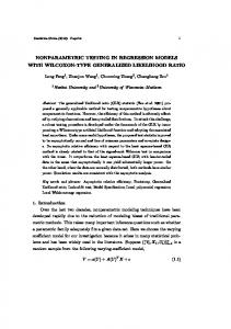
Noninferiority designs are useful when the goal is to demonstrate that a preferred treatment is “at least as good as” or “not worse than” a competitor or standard treatment.5,6 For example, if the preferred treatment is less expensive or safer, it would suffice to show it was at least not worse (and perhaps better) than a comparator on the primary measure of efficacy. Also, cost effectiveness might be assessed, for example, by simply requiring noninferiority on either cost or effectiveness, and superiority on the other. Noninferiority was the approach taken in the design and analysis of the companion paper in this issue of the journal by Ruetzler et al.,7 in which researchers tested the hypothesis that intraoperative distal esophageal (core) temperatures are not !0.5°C lower (a priori specified noninferiority !) during elective open abdominal surgery under general anesthesia in patients warmed with a warm water sleeve on one arm than with an upper body forced air cover. Patients were randomly assigned to intraoperative warming with either a circulating water sleeve (n " 37) or forced air (n " 34); intraoperative core temperature was measured every 15 minutes, beginning 15 minutes after intubation (Fig. 1). Because temperatures were recorded over time, the Ruetzler et al. trial was a repeated-measures design. We use these data to illustrate various approaches to noninferiority as well as to equivalence and superiority analyses. Throughout this article, we refer to Ruetzler et al. as “the companion paper.” Figure 2 depicts sample CIs and the appropriate inference for the 3 types of designs that we discuss. In a superiority trial the null hypothesis of no difference is only rejected if the observed CI for the treatment difference does not overlap zero. Thus, result A in Figure 2 can claim superiority of test treatment T to standard S, but result B cannot. In a noninferiority trial, one treatment is deemed “not worse” than the other only if the CI for the difference lies above a prespecified noninferiority ! (thus, result C can claim noninferiority, but result D cannot). Finally, in an equivalence trial, 2 treatments are deemed “equivalent” March 2011 • Volume 112 • Number 3
Equivalence and Noninferiority Testing with Repeated Measures
focus on continuous outcomes, we briefly review noninferiority and equivalence testing methods for some additional outcome types. Sample size considerations for these designs are also discussed. Throughout this article, we illustrate our examples with data from the companion paper.
SUPERIORITY, EQUIVALENCE, AND NONINFERIORITY DESIGNS—THE BASICS Superiority Testing
For a study designed to assess superiority of one intervention over another for a continuous outcome, the null and alternative hypotheses are
H0: " E # " S $ 0 and H1: " E # " S % 0,
(1)
where "E and "S are the population means for the respective experimental (E) and standard (S) interventions. Assuming a normal distribution for the outcomes in each group and equal variances, we use the Student t test to assess superiority of E to S (or S to E). The test statistic is
Tsup $
Figure 1. Mean and SD of intraoperative temperature with warm water sleeve and forced air from Ruetzler et al.7
only if the CI falls within the prespecified equivalence region (result E can claim equivalence, but result F cannot). Our goal is to review statistical approaches for equivalence and noninferiority trials in various clinical settings; for comparison, we also briefly present analysis of conventional superiority trials. We first review basic methods for design and analysis of each type of trial.8 –12 We then demonstrate how to analyze these designs in a linear regression model, including the repeated-measures setting in which there are multiple outcomes per subject, as in the companion paper. We give particular attention to assessing the interaction between the repeated factor, which is usually elapsed time in perioperative studies, and the intervention. Although we
Figure 2. Sample confidence intervals (CIs) and inference for trials assessing superiority, noninferiority or equivalence of treatment T to standard S. NI " noninferiority. Notice, for example, that CIs B and C are identical, but that the permitted conclusions quite different because the designs and hypotheses differ. Reprinted with permission and modifications from Mascha (2010).8
March 2011 • Volume 112 • Number 3
!
s p2
"ˆ E # "ˆ S # 1/n E & 1/n S$
,
(2)
where "ˆ E and "ˆ S are the observed means (and "ˆ E%"ˆ S estimates the treatment effect), SP is the pooled estimate of the common SD across groups, where SP $ 1/ 2 #nE # 1$sE2 & #nS # 1$sS2 , sE2 and sS2 are the observed varinE & n S # 2 ances (i.e., squared standard deviations) and nE and nS are the sample sizes for the E and S interventions, respectively. The denominator of Equation (2) is the estimated SD of " ˆE # "ˆ S, also called the estimated SE of the difference, or ˆ SE .
"
#
"ˆ E # "ˆ S
For a 2-sided test of superiority we compare the absolute value of Tsup to a t distribution with nE % nS % 2 degrees of freedom (df) at the '/2 level, where ' (“alpha”) is the a priori specified significance level or type I error for the study, typically 0.05. The 2-sided superiority P value is twice the probability of observing a value greater than $Tsup$ if the null hypothesis were true. The null hypothesis is rejected if the P value is smaller than the designated '. Correspondingly, the null hypothesis is rejected if the 100(1–')% CI does not overlap zero. Our primary outcome in the companion paper was core temperature during surgery. The study was designed as a noninferiority trial; but as an example, we first apply a test of superiority to the dataset. Because the study had a repeated-measures design, with temperature measured every 15 minutes intraoperatively, the dataset has 1 row per subject per repeated measurement, with variables site_id (1 " Cleveland Clinic, 2 " Medical University of Vienna), pt_id " patient ID, sleeve (1 " warming sleeve, 0 " forced air), time_m (minutes after induction), esophtemp (esophageal temperature at specified time) and preoperative temperature. The full dataset is included in Appendix 1, which consists of raw data from the companion paper7 (see Supplemental Digital Content 1, http://links.lww.com/AA/A209) and is available from the authors in Excel and tab-delimited formats.
www.anesthesia-analgesia.org
679
STATISTICAL GRAND ROUNDS
We also supply SAS code (SAS statistical software, Cary, NC) in Appendix 2 (see Supplemental Digital Content 2, http://links.lww.com/AA/A210) to perform most of the presented analyses. To demonstrate this basic superiority analysis, we choose a subject’s intraoperative temperature at 60 minutes after intubation as the primary outcome. Any single-number patient summary could similarly be used such as average intraoperative temperature, maximum temperature, or final intraoperative temperature. Summarizing the 60-minute temperatures within group, we obtain mean (SD) of 35.96°C (0.43°C) and 35.87°C (0.47°C) for the circulating water and forced air groups, respectively. The estimated pooled SD is thus SP $ 1/2 #37 # 1$0.432 & #34 # 1$0.472 $ 0.45. Inserting SP along 37 & 34 # 2 with the observed means into Equation (2), we obtain the T statistic for superiority as
"
#
Tsup $
35.96 # 35.87
!0.45
2
# 1/37 & 1/34 $
$
0.091 0.106
$ 0.86
(3)
Because $0.86$ " 0.86 is smaller than 1.99, the t distribution at 1 %'/2 (or 0.975) with 37 & 34 % 2 " 69 df, we do not reject the null hypothesis of no difference, with a corresponding P value of 0.39 for superiority. Corresponding to the nonsignificant test result, the 95% confidence interval for the difference between means is (%0.12, 0.30), which overlaps the null hypothesis value of zero difference. We stress that lack of significance in a superiority analysis is no basis for a claim of equivalence. It could simply reflect, for example, lack of power due to a small sample size or high variability in the outcome measured.
Equivalence
Special designs and statistical approaches are necessary when the goal is to demonstrate that 2 interventions are equivalent.9,13,14 We test the hypothesis that the difference between interventions falls within an a priori specified equivalence region ranging from %! (“%delta”) to &! (“&delta”), outside of which the interventions are deemed nonequivalent. In an equivalence design, the null hypothesis is thus that the true difference is outside of the equivalence region, as
H0: " E # " S ( # ! OR " E # " S ) & !
(4a)
versus the alternative, which we hope to conclude, that the true difference is within the region, as
H1: " E # " S * # ! and " E # " S + & ! .
(4b)
Two 1-sided tests can be used to test whether the true difference is above %! and also below &!.15 If both tests are significant, the null is rejected and equivalence claimed. More simply, though, equivalence is claimed at the given ' level if the CI for the difference falls within the equivalence region.9 If the two 1-sided tests are both significant, the CI for the difference will fall within the equivalence region, and vice versa. If equivalence had been hypothesized for the 2 interventions in the companion paper, the equivalence region might have been chosen as %0.5°C to &0.5°C for the difference in
680
www.anesthesia-analgesia.org
temperature means. Supposing an a priori ' level of 0.025 had been specified for the study, then each of the lower and upper boundaries of the equivalence region would be tested at an ' of 0.025, and the 100(1 to 2')% " 95% CI for the difference at 60 minutes would be (%0.12°C, &0.30°C), as is reported above in the superiority testing; equivalence would be claimed because the CI falls within (%0.5°C, &0.5°C). In an equivalence design, both tests must be significant in order for equivalence to be claimed. Consequently, no adjustment to the significance criterion for performing 2 tests (such as a Bonferroni correction) is needed or appropriate. Instead, each of the lower and upper tests uses the same overall ' level. However, an interesting feature of an equivalence design is that because each of the 2 boundaries are tested at the overall ' level, the estimated interval is a 100(1 to 2')% CI, or in this example, 95%, because ' is 0.025 for each side.9 If the conventional ' level of 0.05 had been used, we would then have a 90% CI.
Noninferiority
In the companion paper we were not actually interested in equivalence per se because the clinical question was not whether the experimental device warmed as well as the current warming standard, forced air. Instead, the question was whether the new system was at least as good as forced air. We thus sought noninferiority—in other words, that the circulating water sleeve was no worse than forced air, and thus either equivalent or better. Specifically, our null hypothesis was that mean distal esophageal (core) temperature in patients assigned to the circulating water sleeve was )0.5°C lower (i.e., worse) than was mean core temperature in those assigned to forced-air warming. The corresponding alternative hypothesis was that mean intraoperative core temperature was not !0.5°C lower in patients warmed with a warm water sleeve than with an upper body forced-air cover, and perhaps higher. Our primary noninferiority analysis included multiple intraoperative core temperature measurements per patient, as is detailed below. By way of example, we first consider a noninferiority test restricted to a single temperature in each patient recorded 60 minutes after induction, as in the superiority test in Equation (3) above. A noninferiority test is basically a 1-sided equivalence test. When higher values of the outcome are desirable, we test the null hypothesis that the preferred treatment is worse by ! or more against the alternative that it is either better or at least no more than ! worse, as
H0: " E # " S ( # ! versus H1: " E # " S * # !
(5)
with a 1-sided test, conducted at the a priori significance level, ' (typically either 0.05 or 0.025). The noninferiority test is 1-sided because we test only one direction, i.e., that the treatment difference is no smaller than %! (when large values of the outcome are desirable). Expressing H1 as " E # " S & ! * 0 (by moving the ! to the left side in Equation (5)) leads to the t test statistic to assess noninferiority, i.e., whether the difference in means is above the lower limit of %!, as
ANESTHESIA & ANALGESIA
Equivalence and Noninferiority Testing with Repeated Measures
TL $
!S
"ˆ E # "ˆ S & ! 2 p
# 1/n E & 1/n S$
.
(6)
Noninferiority is claimed if TL is larger (because H1 has a “greater than” sign) than the value of T from a t distribution with nE % nS % 2 df at 1 % '. The P value is the probability of observing a larger value of TL if the null hypothesis (i.e., inferiority) were true in the population sampled from. For a P value less than ', we reject H0 and conclude noninferiority, i.e., that "E is no more than ! less than "S. Inserting the estimated group means and standard deviations, the observed test statistic TL becomes
TL $
35.96 # 35.87 & 0.5
!0.45
2
# 1/37 & 1/34 $
$
0.091 & 0.5 0.106
$ 5.6. (7)
Our a priori ' was 0.025, so we compare 5.6 to 1.99, the t distribution at 1 % ' " 0.975 with 37 & 34 to 2 " 69 df. Because 5.6 is larger than 1.99, we reject the null hypothesis and claim noninferiority at a ! of 0.5°C (P value '0.001). Alternatively, when lower values of the outcome variable are desirable, the signs are reversed from above, so that Equation (5) is H0: "E # "S ) ! versus H1: "E # "S + !, the numerator for Equation (6) is " ˆ E # "ˆ S # !, and noninferiority is claimed if TL is smaller (not larger) than the value of T from a t distribution with nE # nS # 2 df. More simply, noninferiority is claimed if the estimated 100(1–')% lower confidence limit is above %! (when higher values are a priori more desirable) or when the upper limit is below &! (when lower values more desirable). In our example the estimated lower 100(1–')% confidence limit for ' " 0.025 is
ˆ "ˆ E # "ˆ S # t 1%.025,69 df # SE "ˆ E # "ˆ S$
regression model to test superiority and noninferiority (for a single outcome), and then discuss a linear mixed-effects model for the repeated-measures setting.
Superiority via Linear Regression Modeling
The outcome Y can be modeled as a function of treatment group in a linear regression model as
Yi $ , 0 & , 1 - treatmenti & ei ,
where Yi is the outcome of interest (here, intraoperative temperature at 60 minutes) for the ith subject; ,0 is the intercept, equal to the mean of Y when treatment " 0; ,2 is the treatment effect, the difference between the mean of Y for treatment and control (i.e., "E %"S); treatmenti is a binary indicator for the ith subject equal to 1 for treatment (circulating water sleeve) and 0 for control (forced air cover), and ei is the error term or residual for the ith subject, i.e., the difference between the model prediction and the observed data. Thus, the mean of Y for a particular group is equal to ,0 when treatment " 0 and the ,0 & ,1 for treatment " 1, and ,1 is the difference. Using the linear regression model in Equation (9), one can describe the null and alternative hypotheses for a superiority test by using the treatment effect ,1 as
H0: , 1 $ 0 versus H1: , 1 % 0.
HYPOTHESIS TESTING WITHIN A REGRESSION MODEL
One of the basic tests described in the previous section is often all that is needed to assess either superiority, noninferiority, or equivalence. However, an analogous regression modeling approach is helpful in certain situations. For example, one might want to adjust for imperfectly balanced baseline variables to avoid confounding. Adjusting for baseline variables usually improves precision of the treatment effect estimate to the extent that the variables are correlated with a continuous outcome. Precision can also often be gained by adjusting for the baseline value of the outcome variable itself.16 Finally, a regression model is often a good approach for a repeated-measures setting. Again, using continuous outcomes, we begin with a linear
March 2011 • Volume 112 • Number 3
(10)
From standard statistical software we obtain a treatment ˆ ˆ .When no addieffect estimate ,ˆ and its estimated SE 1
,1
tional covariables are included in Equation (9), ,ˆ 1 is equivalent to " ˆ E # "ˆ S, the observed difference in means, and ˆ ˆ is equal to S 2 # 1/n & 1/n $ . For a 2-sided superiorSE
!
,1
E
p
S
ity test we then assess whether the difference in means is greater than zero, using the test statistic
TS $
"0.091%1.99(.106)"%0.12. (8) Because %0.12 is above the %! value of %0.5, noninferiority is concluded for the circulating water sleeve in comparison with forced air at the 0.025 significance level. A significant noninferiority test (as in Equation (7)) will coincide with the lower end of the estimated CI being above the specified %! (or below &! if lower values of the outcome are desirable).
(9)
!
"ˆ E # "ˆ S
S p2
# 1/n E & 1/n S$
$
,ˆ 1 ˆ SE ,1
,
(11)
and comparing the absolute value of TS to a t distribution with nE % nS % 2 df as in Equation (2). Inserting temperatures from the companion paper at 60 minutes after intubation to the regression model in Equation (9), we obtain ˆ $ 0.106 , estimates ,ˆ $ 35.87 , ,ˆ $ 0.091 , and SE 0
1
,1
resulting in an equation to estimate means for either group as Mean Yi " 35.87 & 0.091 ( Treatment (0 or 1) and a superiority test identical to Equation (3). With the same P value of 0.39, we do not reject the null hypothesis of equal means. In general, a linear regression model approach comparing groups on a single outcome with no additional covariables gives results identical to the simple approaches discussed above—for superiority, noninferiority, or equivalence designs—and has similar assumptions (normality of the residuals and equal variances of the residuals for the 2 groups). However, perhaps the most common reason for using a regression approach is to include covariables in the model to increase precision, adjust for confounding, test for interactions, and assess the association of these variables with the outcome. In such cases, inference on the main
www.anesthesia-analgesia.org
681
STATISTICAL GRAND ROUNDS
effect of interest, the treatment effect, would still be assessed using ,ˆ 1and its SE as in Equation (11), although the estimates might be attenuated by the addition of the covariables (e.g., when adjusting for confounders).
Noninferiority from Same Linear Regression Model
For noninferiority, the hypotheses using the modeling approach are the same as in Equation (5), with the treatment effect expressed as ,1, and with the null hypothesis H0: ,1 ( %! versus the alternative H1: ,1 ! %!. The same linear regression model as for superiority testing in Equation (9) is used to obtain estimates of treatment effect and SE, and the noninferiority ! is added to the test statistic as
TNI $
"ˆ E # "ˆ S & !
!S #1/n 2 p
E
& 1/n S$
$
,ˆ 1 & ! ˆˆ SE ,1
.
(12)
In this basic case (no covariables, and the outcome Y being individual temperatures at 60 elapsed minutes), the resulting test for noninferiority and CI for the difference are exactly as in Equation (7).
Repeated-Measures Designs
We first give an overview and discuss some unique features of a repeated-measures design and analysis and then demonstrate assessment of noninferiority in such a design with results from the companion paper. Analyzing repeated-measures data. In studies of perioperative management, it is often intuitive to assess the effect of treatment across a range of measurement times or other within-subject factors. Such repeated-measures designs have the benefit of usually increasing power over studies with a single outcome measurement by decreasing the SE of the treatment effect. When the outcome consists of repeated measurements on the individual patients, noninferiority (or equivalence or superiority, depending on the design) can be assessed by tests analogous to the models above. Some unique features of a repeated-measures design and analysis are the data setup, the within-subject correlation across the repeated measures, and the potential interaction between treatment effect and the repeated factor (elapsed time in our example). Crossover or paired-data designs,17,18 in which the treatment itself (perhaps anesthetic dose or type) is the repeated factor, can also be analyzed in the repeated-measures framework. We focus, however, on 2-group parallel designs in which the repeated factor is distinct from the treatment or intervention factor. Most statistical programs require data for a repeatedmeasures analysis to have a single row per subject per repeated measurement, with variables for identification (ID), treatment, time, and outcome. Any included covariables are included in additional columns. The online Appendix 1 (http://links.lww.com/AA/A209) contains the data and layout for the companion paper analysis. Measurements within a subject are likely to be more similar than are measurements between subjects. Consequently, within-subject correlation must be considered in the design and analysis of a repeated-measures design. We cannot assume all data points to be independent as we do
682
www.anesthesia-analgesia.org
when there is one observation per subject. In the companion paper, temperature measurements were planned to be taken for each patient at the same 15-minute intervals starting 15 minutes after induction, through 240 minutes. We therefore planned for and used a linear mixed-effects model19,20 (using the Mixed procedure in SAS statistical software),21 in which we estimated a common (i.e., exchangeable) correlation between all pairs of within-subject measurements. Other viable options for the correlation structure would have been autoregressive (i.e., assuming less correlation for times farther apart) and unstructured (i.e., a distinct correlation for every pair of measurement times). The estimates for the chosen correlation structure are modeled in what is termed the “R” matrix, and specified in the SAS Mixed procedure, for example, using the “repeated” statement. Besides allowing assessment of fixed effects (e.g., intervention, age, body mass index) as in simple linear regression, and adjusting for within-subject correlation through the R matrix, the linear mixed-effects model can incorporate extra variation in an outcome due to random effects, i.e., variables with multiple, correlated observations within unit (such as patient, anesthesiologist, or clinical site), for which the observed units are typically only a subset of the desired inference. Alternatively, a patient’s deviation from an estimated mean slope of an outcome measured over time, or a patient’s deviation from the overall intercept (i.e., the outcome value at time zero of the regression line), can be modeled as a random effect. Variation in the outcome due to random effects is modeled in the “G” matrix, and specified in SAS Mixed procedure, for example, using the “random” statement.22 For the companion paper, no random effects other than the default error term were explicitly modeled, because within-subject correlation was accounted for in the R matrix. For example, extra variation due to clinical site was so negligible that no variance for this potential random effect could be estimated. In practice, linear mixed-effects modeling has largely replaced the traditional “repeated-measures analysis of variance (ANOVA)” for repeated-measures designs. One major reason is that whereas the traditional method requires all patients to be measured at the same time points and with no missing data, mixed-effects modeling allows for differing numbers of measurements and different measurement times for each subject, as well as data that are missing at random. The linear mixed-effects model is thus considerably more practical for intraoperative studies, in which patients may or may not have regularly scheduled measurements, but certainly have operations of varying lengths. For example, patients in the companion paper had a median (quartiles) of 15(12,16) temperature measurements, but 14 of 71 patients had 10 measurements or fewer. Most of the variability in the number of measurements came from differing lengths of surgery, but some patients had missing data for some of the 15-minute time intervals. The mixed-effects model can also handle the common case (especially in retrospective studies) in which no 2 patients are measured at the same time points. In addition, whereas the traditional model requires the same correlation for all pairs of measurements, the linear mixed-effects model
ANESTHESIA & ANALGESIA
Equivalence and Noninferiority Testing with Repeated Measures
allows estimation of random effects and a wide variety of flexible within-subject correlation structures. Flexibility regarding the number of measurements per patient is a main strength of the linear mixed-effects model, but it is also usually optimal for comparative groups to have a similar mean number of measurements per patient. First, the linear mixed-effects model gives more weight to patients having more measurements, and second, a substantial difference between groups in the average number of measurements per patient may make inference between the groups difficult. For example, a linear mixed-effects model comparing groups on intraoperative glucose levels in which glucose was measured every 15 minutes in the experimental group but much less frequently (every 60 minutes on average) in the standard care group would give more weight to the experimental group patients and be more accurate in summarizing the glucose pattern of the experimental than the standard care patients. The relationship between time (or whatever the repeated factor) and outcome may be of interest in itself, but in a comparative intervention study it is usually included in the model to remove an important source of variance and to assess interaction with treatment. Time can be modeled along with the treatment effect as
Yij $ ,0 & ,1 treatmenti & , 2 timej & eij,
(13)
where Yij is the observed temperature for the ith subject at the jth time, and eij is the error term. The repeated factor can be modeled either as a continuous variable as in Equation (13) or as a categorical factor for which binary indicator variables for each level (here, each time point) except the reference level are entered into the model. Choice depends on the research question and the observed shape of the data. Time modeled as a continuous variable enables estimation of the average change in outcome per unit time, and is most appropriate when a linear increase or decrease is expected and observed, and the categorical option is useful if it is clear that the outcome does not follow a linear pattern over time, or if comparisons among the times or among treatments at specific times are of interest. It is often of interest to assess the interaction between treatment and time. If the hypothesis is that one method is noninferior (or superior or equivalent, again depending on the design) to the comparator method at any of the measured times, we first assess whether the treatment effect is consistent over time by testing for a Treatment ( Time interaction. There is an interaction whenever the effect of one factor depends on the level of another. For example, some evidence for a Treatment ( Time interaction is present in Figure 1, where mean core temperature with the warm water sleeve appears to be the same or slightly lower than the comparator at early times but higher than the comparator at later times. If no Treatment ( Time interaction is detected, the overall treatment effect can be assessed marginally, that is, by collapsing over time. This is done by fitting a model as in Equation (13) to assess the treatment effect while adjusting for time in the same model. If time is categorical and all patients have the same number of measurements, the marginal approach is equivalent to taking the arithmetic average of all the temperatures in each patient, and then
March 2011 • Volume 112 • Number 3
conducting a simple t test (for noninferiority or superiority) on the patient averages using the methods above. If the interaction is statistically and clinically significant, and particularly if there is a qualitative interaction (i.e., the direction of treatment effect varies across the times) versus quantitative interaction (i.e., effects are in same direction but vary only in degree over time), the treatment effect should be assessed at specific time points and not overall. With time as a continuous variable, the Treatment ( Time interaction is assessed by testing whether ,3 in the following model is equal to zero:
Yij $ ,0 & , 1 treatmenti & , 2 timej &
, 3 treatmenti - timej & eij.
(14)
However, in certain situations the Treatment ( Time interaction is irrelevant because it does not matter at which point in time a patient’s values were increased (or decreased); a summary of each patient’s values over the relevant time interval is the primary interest. Here the primary outcome can be a single value consisting of the patient average or the time-weighted average and tested via a simple t test as in Equation (4) for equivalence or Equation (5) for noninferiority. The time-weighted average approach directly accounts for time between measurements and is particularly useful if the times are not equidistant, in which case the simple average or repeated-measures approach may not be appropriate. If times are equidistant, then the time-weighted-average approach gives the same result as does the simple average, and the same as the linear mixed-model approach with equal numbers of measurements per patient and no Treatment ( Time interaction specified. Noninferiority in a repeated-measures design. In the companion paper we in fact wanted to make conclusions about the noninferiority of circulating water sleeve versus forced-air warming at specific times during the surgery. Therefore, a patient summary such as time-weighted average was insufficient because that approach would average all within-patient temperatures before the model was constructed. We thus needed a repeated-measures model to assess whether the treatment effect was consistent across surgical times by testing for a Treatment ( Time interaction. As was mentioned, we used a linear mixed-effects model with a common “exchangeable” correlation, such that a single correlation coefficient of 0.71 was estimated for all pairs of time points within subjects. Although an autoregressive structure may have been a more natural choice and a somewhat better fit to the data, because measurements closer together within a patient may be expected to be more correlated than would those farther apart, results were quite similar with either method and the conclusions were the same. With the autoregressive structure the estimated correlations ranged from 0.96 for adjacent pairs of measurements to 0.56 for the measurements farthest apart. An unstructured correlation model was not possible because of the large number of measurements per patient, but is generally a good choice when there are relatively few repeated measurements in relation to the number of patients. A plot of temperature over time for the 2 randomized groups showed that temperature did not have a linear
www.anesthesia-analgesia.org
683
STATISTICAL GRAND ROUNDS
Table 1. Testing Noninferiority of the Warm Water Sleeve to Forced Air Elapsed hour (N: WW, FA) 1 (37, 34) 2 (31, 32) 3 (26, 29) 4 (18, 20)
Warm water mean (SE) 35.96 (0.081) 36.06 (0.084) 36.16 (0.087) 36.25 (0.094)
Forced air mean (SE) 35.87 (0.085) 36.09 (0.086) 36.37 (0.087) 36.46 (0.094)
Difference (95% CI)a 0.09 (%0.14, 0.31) %0.03 (%0.26, 0.21) %0.21 (%0.45, 0.03) %.0.21 (%0.47, 0.06)
Significance criterionb 0.0062 0.0083 0.0125 0.0250
P valuec '0.0001 '0.0001 0.011 0.016
WW " warm water sleeve; FA " forced air; SE " standard error; CI " confidence interval; NI " noninferiority. a Difference " mean WW minus mean FA. Normally, NI concluded if the lower 95% confidence limit is above NI delta of %0.5°C. Here, we also need P values to be less than the given Holm–Bonferroni significance criterion. b Holm–Bonferroni method23: significance criterion for smallest P value " 0.025/k, where k " 4 tests; next smallest P value criterion is 0.025/(k % 1), etc. c P value from 1-tailed test for NI using linear mixed model: all are noninferior because each P value is less than criterion.
relationship with time: instead, it decreased in both groups for the first hour, and then progressively increased through the remaining 4 study hours (Fig. 1). For our main analysis, we therefore considered each time point to be a different category, instead of modeling time as a single continuous variable as in Equations (13) and (14). The model thus included variables for treatment group, categories of time, and the Treatment ( Time interaction. By listing time as a categorical or “class” variable, most statistical programs will automatically create the required design variables for the time effect (i.e., design variables time30 through time240 for each 15 minutes of elapsed time, excluding time15, because the first measurement was the reference time), and the Treatment ( Time interaction terms as
Yij $ ,0 & , 1 TXi & , 2B time30 & , 2C time45 &
, 2D time60 & … & , 2P time240 & , 3B TXi - time30 & , 3C TXi - time45 & … & , 3P TXi - time240 & eij.
(15)
We assessed the Treatment ( Time interaction by testing whether the vector of interaction terms ,3B % ,3P was equal to zero for the model in Equation (15) using an F test, a default statistical software output from such a model. The interaction was highly significant at P ' 0.001 (for either categorical or continuous time), implying a nonconsistent treatment effect over the times. We therefore followed with separate assessments of noninferiority for elapsed hours 1, 2, 3, and 4 of surgery. Direct estimates of the treatment effect at specific times could be derived by specifying “least squares means” for the Treatment ( Time interaction in Equation (15), and then searching the statistical software output for the comparisons of interest. More efficiently, we obtained direct estimates of the treatment effect at specific times using an alternative form of Equation (16) in which we removed the intercept (an option in most statistical software) and the treatment variable, and only included time and Treatment ( Time interaction variables, as in
Yij $ , 2A time15 & , 2B time30 & , 2C time45 &
, 2D time60 & … & , 2P time240 & , 3A TXi - time15 & , 3B TXi - time30 & , 3C TXi - time45 & … & , 3P TXi - time240 & eij. 684
www.anesthesia-analgesia.org
(16)
The estimated betas for the interaction terms in this model directly estimate the difference between groups at each respective time point, and are reported in the Difference column in Table 1 (modified from Table 2 of the companion paper) for hours 1, 2, 3, and 4. We then performed the same noninferiority test as in Equation (12), each time substituting the corresponding estimated treatment effect and SE from the model in Equation (16). Using the Holm–Bonferroni multiple comparison procedure,23 all 4 tests for noninferiority were significant at the respective criterion, and noninferiority of the circulating water sleeve to forced air was concluded at each time point (Table 1). We tested only at each hour because testing every 15 minutes would not be clinically relevant and would thus be an inefficient use of ' (i.e., requiring an overly conservative significance criterion for each test). It is common practice to adjust for the baseline value of a continuous outcome measure because doing so decreases the SE of the treatment effect (thus increasing power) to the extent that the baseline and outcome measurements are positively correlated. This could be done here by adding baseline temperature to models (15) or (16). We considered such an adjustment as a secondary analysis in the companion paper. However, correlations between baseline and temperature at various intraoperative times were either close to zero or negative, and adjusting for a variable negatively correlated with outcome increases the SE of the treatment effect, thus decreasing power. Therefore, no adjustment was made. Clinical site was not related to the outcome (P " 0.94), and there was no evidence of Treatment ( Site interaction (P " 0.88). Similarly, no adjustment for confounding was done because the randomized groups were well balanced on all baseline variables.
EXTENSIONS TO ADDITIONAL OUTCOME TYPES
In addition to continuous outcomes, noninferiority and equivalence testing in both the single outcome and repeated-measures settings can be constructed for most data types4—including binary,4,5,11,24 ordinal,25 nonnormal continuous (extension of Wilcoxon–Mann–Whitney test),4,26 and survival outcomes11,27— by adapting the usual tests for superiority. Of mention, Tunes da Silva et al.11 give a thorough presentation of binary and survival outcomes. For nonnormal continuous or ordinal outcomes, noninferiority and equivalence tests can be based on the fact that the Wilcoxon–Mann–Whitney test for superiority actually tests the probability P& that a randomly chosen subject
ANESTHESIA & ANALGESIA
Equivalence and Noninferiority Testing with Repeated Measures
from the experimental group E has a higher (or lower) outcome value than does a randomly chosen subject from group S, with null hypothesis H0: P& " 0.5 (i.e., E and S subjects equally likely to have higher values). For noninferiority, then, the null and alternative hypotheses when higher values of the outcome are desirable can be specified as
H0: P & ( 0.5 # ! vs H1: P & * 0.5 # ! ,
(17)
where ! is the deviation from a probability of 0.5 chosen to define the noninferiority region. Construction of the test for noninferiority can be done using a 1-sided version of the equivalence test outlined in Wellek (chapter 6) for nonnormal continuous outcomes.4 For binary outcomes, basic noninferiority and equivalence testing involves substituting proportions for means and the SE of the difference in proportions for the difference in means, with ! specified as an absolute difference in proportions.5,11 Alternatively, the noninferiority or equivalence ! can be expressed as a ratio of 2 proportions, or relative risk. For example, suppose we want to assess whether success with preferred treatment E is not worse than that with standard S. A null hypothesis for noninferiority could be that the success proportion (P) with E is at least 10% less than that for S, for a ratio ! of 0.9, and H0: PE/PS ( 0.90. The alternative would be that the success ratio is !0.90, or H1: PE/PS ! 0.90. Using algebra, H1 can be expressed as H1: PE % 0.9 PS ! 0, and a test statistic for noninferiority would be
TL $
pˆ E # ! pˆ S
!pˆ #1 # pˆ $/n E
E
E
& pˆ S# 1 # pˆ S$ ! 2/n S
,
(18)
where pˆ E and pˆ S are the observed success proportions for treatments E and S, respectively, and ! is the minimum ratio of proportions deemed to be “not worse.” When the ratio ! is '1.0, i.e., when a higher outcome proportion is desirable, noninferiority testing using the ratio formulation in Equation (18) is always more efficient (smaller SE due to !2 in denominator) than is the traditional approach5 of specifying the ! as an absolute difference in proportions and using the formula analogous to Equation (6).24 When a lower outcome proportion is desirable, the hypotheses can be rearranged to make ! '1.0. As in the traditional approach for dichotomous outcomes, noninferiority testing using Equation (18) can be used whenever the proportions are not extremely close to 0 or 1 and the sample size is large enough to assume the proportions are approximately normally distributed, typically when np ! 5 and n(1 % p) ! 5 (where p refers to each of PE and PS, and n refers to each of nE and nS). In a repeated-measures design with binary outcome, noninferiority or equivalence can be assessed using a generalized estimating equation28,29 or generalized linear mixed-model approach30 to account for the within-subject correlation by using methods analogous to those above. A noninferiority ! can also be expressed as a minimal odds ratio (when the binary outcome event is desirable (i.e., success)), for which treatment E is not worse than treatment S, and testing occurs on the log-odds ratio scale. The CI approach would claim noninferiority if the lower
March 2011 • Volume 112 • Number 3
100(1–')% confidence limit was above the odds ratio !. Of note, however, the absolute difference in proportions implied by a particular odds ratio or relative risk depends heavily on the control group success proportion. Therefore, care must be taken to assure that the chosen odds ratio or relative risk ! implies a clinically relevant difference in proportions.11
SAMPLE SIZE CONSIDERATIONS
For noninferiority testing, sample size calculations are the same as those for a 1-tailed test for superiority when the specified ! is the same as the superiority population difference to detect. We stress, though, that a noninferiority ! for a comparative efficacy study should be considerably smaller than a specified population difference used to assess superiority of a treatment versus placebo. For this reason, noninferiority trials usually require more patients than do superiority trials.31 Per-group sample size for a noninferiority design is
n$
2 #Z1 # ' & Z 1 # , $2 .2
!2
(19)
where Z1%' and Z1%, are the standard normal deviates corresponding to 1 minus the significance level (') and 1 minus the type II error (,), respectively, .2 is the variance or squared SD of the outcome, and ! is the noninferiority !.11 For example, for ' " 0.05, , " 0.10, . " 0.5, and a noninferiority ! of 0.25, sample size per group would be 2 # 1.645 & 1.28 $ 20.5 2 n $ $ 69. Alternatively, with ' " 0.25 2 0.025 (so that z " 1.96), the resulting sample size is n " 84 per group. The superiority formula (2-tailed test) replaces Z1%' with Z1%'/2. In an equivalence trial, multiple comparison adjustments for performing the two 1-sided tests are unnecessary because both tests must be significant to claim equivalence, and only one conclusion is made (equivalence claimed or not claimed). However, because both tests must be significant to detect a treatment effect that lies between the 2 boundaries, the most appropriate sample size formula includes the standardized normal deviate (Z) corresponding to “1 minus ,/2” instead of “1 minus ,“ as in noninferiority or superiority testing. Sample size for a given ', !, and power is thus higher for an equivalence design than for a noninferiority design.32 For repeated-measures designs, accurate sample size calculations require estimation of the degree and structure of the within-subject correlation, along with the average number of measurements per subject (in addition to ', ,, SD, and !). When the repeated factor is distinct from the intervention factor, as in the companion paper, lower within-subject correlations across the repeated factor and more observations per subject both decrease the required sample size.33,34 It remains important though, in repeated-measures designs, to plan for sufficient power to detect group differences at particular levels of the repeated factor in the presence of a Treatment ( Repeated Factor interaction. In the companion paper, for example, we planned for 90% power at the 0.025 significance level to detect noninferiority
www.anesthesia-analgesia.org
685
STATISTICAL GRAND ROUNDS
of the warming sleeve to forced air with an SD of 0.6°C and noninferiority ! of 0.6°C. Although this calculation, resulting in 32 patients per group, was conservative by ignoring the added power inherent in the repeated-measures design, it would have been quite appropriate to calculate the sample size assuming group comparisons at the 4 individual time points due to the possible (and realized!) Treatment ( Time interaction, thus using an ' of 0.025/4 " 0.00625 in the calculations.
DISCUSSION
Claims of equivalence or noninferiority can only be made in studies specifically designed to assess them, and in which the null hypothesis of lack of equivalence or noninferiority is rejected in favor of the a priori defined alternative.5 Such claims are accompanied by the CI for the treatment effect falling either within the prespecified equivalence region or above the prespecified noninferiority !. It is thus not valid to assess noninferiority or equivalence in a study designed for superiority, even though it might be tempting to “rescue” a negative test of superiority by concluding equivalence, “similarity,” or noninferiority, or perhaps by even choosing an a posteriori ! that fits the observed data! Choosing an appropriate a priori ! for an equivalence or noninferiority study is key, because the ! is an integral part of the hypothesis and is also used in the data analyses.35,36 The need for a defined ! differs from superiority trials in which the anticipated treatment effect is only used for sample size calculations. Choice of ! should be given careful thought, because the selected value will have enormous impact on sample size and interpretation of the observed results. An equivalence ! should be considerably smaller than the “clinically important difference” that would be used in a power analysis for assessing superiority of treatment versus placebo,9 and rationale for the chosen ! should be explained. For example, the companion article by Ruetzler et al.7 states that a ! of 0.5°C was chosen for assessment of noninferiority because no clinically important differences had been seen in previous studies when the average temperature differed by '0.5°C. A ! that is too large promotes false claims of equivalence or noninferiority, whereas too small a ! inflates the sample size, thus adding cost to a study and prolonging the time required to accrue subjects. The general rule is to use a ! that is clinically unimportant, based either on clinical experience or previous work showing that a given ! is unlikely to be associated with substantial differences in important outcomes.37 We demonstrate methods for noninferiority and equivalence testing in the context of a regression model, and in doing so highlight design and analytic features of repeated-measures designs, including incorporation of the within-subject correlation and the importance of the Treatment ( Time interaction. Use of a linear mixedeffects model allows specification of the within-subject correlation and estimation of random effects. It is much more flexible than the traditional repeated-measures ANOVA, because differing numbers of repeated measurements are permitted across subjects (thus including some tolerance for missing data and the natural variability in surgery lengths) and a host of correlation structures may be
686
www.anesthesia-analgesia.org
considered. For example, correlation between measurements that are closer together in time can be estimated distinctly from measurements farther apart. In addition, models can be fit in which a patient’s deviation from an estimate common slope or intercept is treated as a random effect. For these reasons, the traditional repeated-measures ANOVA has been largely replaced by the linear mixed-effects model. Paramount to any noninferiority or equivalence design is a detailed analysis plan that addresses the study hypotheses and provides contingency analysis plans in case data assumptions are not met. Particularly, a repeated-measures design should specify the role of time (or whatever the repeated factor) and its relationship with the treatment effect. For example, if conclusions such as “treatment A is noninferior to treatment B at any time measured” are desired, then assessment of the Treatment ( Time interaction should be planned. Comparisons at specific time points (with adjustment for type I error) should be planned to follow if the interaction is significant; otherwise, the “marginal” treatment effect would be assessed by collapsing over time, which is the more powerful analysis because all data are used in a single comparison. On the other hand, if the timing of a patient’s increased or decreased outcomes is unimportant, the Treatment ( Time interaction may be deemed irrelevant in the planning stage, and the time-weighted average or other withinpatient summary measure chosen as the primary outcome. The time-weighted average gives a single-number subjectspecific summary, while accounting for uneven spacing of measurements, gives equal weight to each subject and reduces the analysis to a simple t test instead of the more complex repeated-measures analysis. It is thus usually preferable to the simple average of a subject’s measurements. Other choices might be the maximum, minimum, or median value of the outcome for a subject. The singlenumber summary should be the outcome measure that best represents the study hypothesis. In summary, proper design of clinical studies depends critically on the type of conclusions investigators will want to make, including potential claims of superiority, noninferiority, or equivalence. Each design has specific implications for formulation of the hypotheses, the corresponding analytic methods,12,38 and reporting (see revised CONSORT statement for equivalence and noninferiority designs).9 Thoughtful choice of the equivalence or noninferiority ! is a critical step in these designs because the a priori ! is used directly in the analyses and interpretation of results. Simple univariable analyses will be appropriate in many circumstances and are easy to implement. But, as is shown, each of the discussed designs can be analyzed in a regression model, thus facilitating covariable adjustment, interaction assessment, and repeated-measures analyses. DISCLOSURES
Name: Edward J. Mascha, PhD. Contribution: This author helped design the study, conduct the study, analyze the data, and write the manuscript. Attestation: Edward J. Mascha approved the final manuscript. Name: Daniel I. Sessler, MD. Contribution: This author helped write the manuscript. Attestation: Daniel I. Sessler approved the final manuscript.
ANESTHESIA & ANALGESIA
Equivalence and Noninferiority Testing with Repeated Measures
REFERENCES 1. O’Connor AB. Building comparative efficacy and tolerability into the FDA approval process. JAMA 2010;303:979 – 80 2. Malozowski S. Comparative efficacy: what we know, what we need to know, and how we can get there. Ann Intern Med 2008;148:702–3 3. Altman DG, Bland JM. Absence of evidence is not evidence of absence. Biometrical J 1995;311:485 4. Wellek S. Testing Statistical Hypotheses of Equivalence. Boca Raton, FL: Chapman and Hall/CRC Press LCC, 2003 5. Blackwelder W. “Proving the null hypothesis” in clinical trials. Control Clin Trials 1982;3:345–53 6. Laster LL, Johnson MF. Non-inferiority trials: the ‘at least as good as’ criterion. Stat Med 2003;22:187–200 7. Ruetzler K, Kovaci B, Guloglu E, Kabon B, Fleischmann E, Kurz A, Mascha E, Dietz D, Remzi F, Sessler D. Forced-air and a novel patient-warming system (vitalHEAT vH2) comparably maintain normothermia during open abdominal surgery. Anesth Analg 2011;112:608 –14 8. Mascha EJ. Equivalence and noninferiority testing in anesthesiology research. Anesthesiology 2010;113:779 – 81 9. Piaggio G, Elbourne DR, Altman DG, Pocock SJ, Evans SJW, for the CG. Reporting of noninferiority and equivalence randomized trials: an extension of the CONSORT statement. JAMA 2006;295:1152– 60 10. Christensen E. Methodology of superiority vs. equivalence trials and non-inferiority trials. J Hepatol 2007;46:947–54 11. Tunes da Silva G, Logan BR, Klein JP. Methods for equivalence and noninferiority testing. Biol Blood Marrow Transplant 2008;15:120 –7 12. Tamayo-Sarver J, Albert JM, Tamayo-Sarver M, Cydulka R. Advanced statistics: how to determine whether your intervention is different, at least as effective as, or equivalent: a basic introduction. J Academic Emergency Med 2005;12:536 – 42 13. Jones B, Jarvis P, Lewis JA, Ebbutt AF. Trials to assess equivalence: the importance of rigorous methods. Biometrical J 1996;313:36 –9 14. Ebbutt AF, Frith L. Practical issues in equivalence trials. Stat Med 1998;17:1691–701 15. Schuirmann D. A comparison of the two one-sided tests procedure and the power approach for assessing the equivalence of coverage bioavailability. J Pharmacokinet Biopharm 1987;15:657– 80 16. Pocock SAS, Enos L, Kasten L. Subgroup analysis, covariate adjustment and baseline comparisons in clinical trial reporting: current practice and problems. Stat Med 2002;21:2917–30 17. Burns DR, Elswick RK. Equivalence testing with dental clinical trials. J Dent Res 2001;80:1513–7 18. Tango T. Equivalence test and confidence interval for the difference in proportions for the paired-sample design. Stat Med 1998;17:891–908
March 2011 • Volume 112 • Number 3
19. Laird NM, Ware JH. Random-effects models for longitudinal data. Biometrics 1982;38:963–74 20. Henderson CR. Applications of Linear Models in Animal Breeding. Guelph, Ontario, Canada: University of Guelph, 1984 21. Littell RC, Milliken GA, Stroup WW, Wolfinger RD, Schabenberber O. SAS for Mixed Models. 2nd ed. Cary, NC: SAS Institute Inc., 2006 22. Krueger C, Tian L. A comparison of the general linear mixed model and repeated measures ANOVA using a dataset with multiple missing data points. Biolog Res Nurs 2004;6:151–7 23. Holm S. A simple sequentially rejective multiple test procedure. Scand J Statistics 1979;6:65–70 24. Laster L, Johnson MF, Kotler ML. Non-inferiority trials: the ‘at least as good as’ criterion with dichotomous data. Stat Med 2006;25:1115–30 25. Wellek S. Statistical methods for the analysis of two-arm non-inferiority trials with binary outcomes. Biometrical J 2005;47:48 – 61 26. Chow SC, Liu J. Design and Analysis of Bioavailability and Bioequivalence Studies. New York: Marcel Dekker, 1992 27. Com-Nougue C, Rodary C, Patte C. How to establish equivalence when data are censored: a randomized trial of treatments for B non-Hodgkin lymphoma. Stat Med 1993;12:1353– 64 28. Liang K-Y, Zeger SL. Longitudinal data analysis using generalized linear models. Biometrika 1986;73:13–22 29. Zeger SL, Liang K-Y. Longitudinal data analysis for discrete and continuous outcomes. Biometrics 1986;42:121–30 30. Vonesh EF, Chinchilli VM. Linear and Nonlinear Models for the Analysis of Repeated Measurements. New York: Marcel Dekker, 1997 31. Snapinn SM. Noninferiority trials (Commentary). Curr Control Trials Cardiovasc Med 2000;1:19 –21 32. Farrington CP, Manning G. Test statistics and sample size formulae for comparative binomial trials with null hypothesis of non-zero risk difference or non-unity relative risk. Stat Med 1990;9:1447–54 33. Verbeke G, Molenberghs G. Linear mixed models for longitudinal data. New York: Springer, 2000 34. Dahmen G, Rochon J, Ko¨nig IR, Ziegler A. Sample size calculations for controlled clinical trials using generalized estimating equations (GEE). Methods Inf Med 2004;43:451– 6 35. Hou Y. Issues on the selection of non-inferiority margin in clinical trials. Chinese Medical J 2009;122:466 –70 36. Wiens BL. Choosing an equivalence limit for noninferiority or equivalence studies. Control Clin Trials 2002;23:2–14 37. Lange S, Freitag G. Special invited papers section: therapeutic equivalence— clinical issues and statistical methodology in noninferiority trials. Biometrical J 2005;47:12–27 38. Kaji A, Lewis R. Are we looking for superiority, equivalence, or noninferiority? Asking the right question and answering it correctly. Ann Emerg Med 2010;55:408 –11
www.anesthesia-analgesia.org
687