Estimating Functional Coverage in Bounded Model Checking

Estimating Functional Coverage in Bounded Model Checking Daniel Große Ulrich K¨uhne Rolf Drechsler Institute of Computer Science, University of Bremen, 28359 Bremen, Germany {grosse, ulrichk, drechsle}@informatik.uni-bremen.de

Abstract Formal verification is an important issue in circuit and system design. In this context, Bounded Model Checking (BMC) is one of the most successful techniques. But even if all specified properties can be verified, it is difficult to determine whether they cover the complete functional behavior of a design. We propose a pragmatic approach to estimate coverage in BMC. The approach can easily be integrated in a BMC tool with only minor changes. In our approach, a coverage property is generated for each important signal. If the considered properties do not describe the signal’s entire behavior, the coverage property fails and a counter-example is generated. From the counter-example an uncovered scenario can be derived. In this way the approach also helps in design understanding. Our method is demonstrated on a RISC CPU. Based on the results we identified coverage gaps. We were able to close all of them and achieved 100% functional coverage.

1. Introduction Today, formal verification is standard in many industrial design flows. One prominent technique in this context is Model Checking (MC) [11]. Model checking is an automatic method for verifying that a finite state system satisfies a temporal property. In Symbolic Model Checking [7, 6] Binary Decision Diagrams (BDDs) [5] are used to represent the state space symbolically. This approach has been used successfully in practice. However BDDs may suffer from the memory explosion. As an alternative Boolean Satisfiability (SAT) based methods have been proposed. In Bounded Model Checking (BMC) [4] the system is unfolded for k time frames and together with the property converted into a SAT problem. If the corresponding SAT instance is satisfiable a counter-example of length k has been found. Due to significant improvements in the tools for SAT solving SAT-based MC methods can be applied to large designs and are widely used in industry [18, 3]. In MC the functional properties are specified in temporal logic. Thus, each property describes parts of the circuit’s behavior unambiguously. However the most important question that arises here is ”have I written enough properties?” [17]. In simulation-based verification computing

coverage is well understood since coverage corresponds to an activation during the execution of input vectors. Also formal techniques have been used to analyze test-benches with respect to functional coverage [12]. For MC estimating coverage is more difficult since the correspondence of coverage is not obvious because the complete underlying Finite State Machine (FSM) is traversed during the proof. Nevertheless there exist several notions of coverage for model checking [9]. For CTL-based approaches the covered states of the FSM are computed [15, 16]. By mutation-based coverage modifications are applied to the FSM and it is checked if this is detected by the specified properties [8, 9]. But most of the existing metrics suffer from complexity problems as in the case of CTL model checking or are still very hard to use by verification engineers in practice. Recently, a first approach for measuring the coverage for BMC has been proposed in [13]. There the focus is mainly to relate errors in the design to the source code level. A component is considered covered, if there is a at least one property that is invalidated, if this component is changed. The notion of “change” is described using a multiplexor construct based on the ideas of [2]. The approach cannot specify exact functional coverage. Instead, components are identified that influence the behavior of the circuit. Thus, the approach cannot present the uncovered scenarios in form of counter-examples. In [10] a method for coverage analysis of safety property lists has been presented. This method works only on the specified LTL properties without using the design. The properties are synthesized into a checker circuit that has exactly one output. This output is 1 iff all properties hold. Then, the checker circuit is duplicated. The two checker circuits use the same variables except for the output signal that is analyzed in the current step. Based on this construction the method can identify a forgotten case, i.e. a trace where a particular output signal is not constrained by the properties. Therefore the method looks for traces where both checker outputs are 1, but the values of the analyzed output signal differ at exactly one time point. The presented method is efficient because the design is not needed. However, if the method has identified a forgotten case there is no information about the circuit behavior. Furthermore the method needs to introduce a new LTL construct for specifying that a signal is allowed to be unconstrained in a certain case.

In this paper we propose a pragmatic approach for the estimation of coverage in BMC. The basic idea is the following: First, for each output o of the circuit all proven properties are identified which argue over o. Then it is checked whether there exists a scenario where o is not determined by the set of properties. Here, not determined means that an input and state assignment has been found where no consequent of the set of properties specifies the value of o unambiguously. We show that this idea can be integrated easily in a BMC verification tool. Furthermore the approach automatically generates uncovered scenarios in form of counterexamples. Analyzing these counter-examples and adding corresponding properties allows the verification engineer to stepwise close the coverage gap. The rest of the paper is structured as follows. In Section 2 BMC is briefly reviewed. Section 3 describes the new approach for estimating coverage in BMC. Then, in the next section experimental results on the formal verification and coverage estimation of a RISC CPU are provided. Finally in Section 5 the paper is summarized.

2. Bounded Model Checking In this paper we use BMC as described in [18]. Thus, a property only argues over a finite time interval. For a design with its transition relation Tδ , a BMC instance for a property p over the finite interval [0, c] is given by: c−1 ^

Tδ (si , si+1 ) ∧ ¬ p

i=0

This verification problem can be formulated as a SAT problem by unrolling the circuit for c time frames and generating logic for the property. In contrast to [4] there is no restriction for the state s0 in the first time frame during the proof. This may lead to false negatives, i.e. counter-examples that start from an unreachable state. In such a case these states are excluded by adding additional assumptions to the property. But, for BMC as used here, it is not necessary to determine the diameter of the underlying sequential circuit, i.e. if the SAT instance is unsatisfiable the property holds. In the following we assume that each property is an implication, i.e. the property has the form A ⇒ C. A is the antecedent and C is the consequent of the property and both consist of a timed expression. A timed expression is formulated on top of variables that are evaluated at different points in time within the time interval [0, c] of the property. The operators in a timed expression are the typical HDL operators, e.g. logic and, logic or, arithmetic operators and relational operators.

3. Estimating Coverage First in this section we provide the basic idea for our coverage approach. Then, we describe our method in detail and discuss the method by using two examples.

3.1. Idea After proving a set of properties the verification engineer wants to know if the properties describe the complete functional behavior of the circuit. Thus, typically the properties are manually reviewed and the verification engineer checks that properties have been specified for each output (and important internal signals) which prove the expected behavior in all possible scenarios. Here, the goal of our approach is to automatically detect scenarios, i.e. assignments to inputs and states, where none of the properties specify the value of the considered output. This idea is realized by the generation of a coverage property for each considered output. If this coverage property holds there exists no scenario where the value of the output o is not determined by the properties. It is shown that the union of all properties that argue over the output o admit no behavior else than the one defined by the circuit. This is done by introducing a multiplexor for each bit that is driven by the output o and the inverted value of o. Then the coverage check can be performed by proving that the multiplexor is forced to select the original value of o, assuming all involved properties. In the following section this is described in more detail.

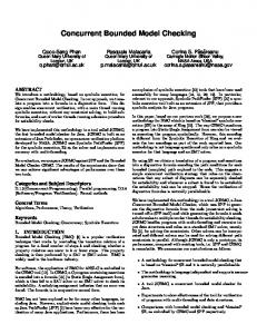
3.2. Coverage Property To estimate the coverage we generate a coverage property for each output o of the design. This coverage property for the output o is constructed as follows: 1. The set of properties Po that argue over the output o is identified. 2. The maximum time point tmax is determined. tmax is defined as the latest time point in the consequent of all properties in Po , at which o is constrained. 3. A multiplexor for each bit of the considered output o is inserted in the original design. Let o consist of the single bit signals o0 , . . . , on−1 . Then, the bit oi of the output is connected to the data input d1 of the i-th multiplexor, whereas the negation of oi is connected to the data input d0 . If o is a single bit signal then we add the new input sel to the design that is connected to sel0 (which is the select input of the multiplexor). Otherwise we add sel0 , . . . , seln−1 as new inputs and the Vn−1 signal sel = i=0 seli . 4. The output o is renamed to o orig and the name of the output of the inserted multiplexor is set to o. Thus in the following all properties that use o are dealing with the output of the multiplexor instead of the originally considered output. The transformation for the single bits of o is depicted in Figure 1. 5. Now the coverage property for the considered output o is generated. In the antecedent all properties of Po are assumed. Possibly a property pi has to be shifted such

we

sel0 o_orig

1

0

0

din

o0

1 0

FF

dout

sel1 o_orig

1

1

0

... Figure 1. Insertion of the multiplexor. that output o in the consequent of pi is constrained at the maximum time point tmax . If the output o is constrained in the consequent of the property pi at m time points with m > 1, then pi is handled as m separate properties, i.e. each such property consists of the antecedent of pi and m different consequents. The resulting properties are denoted as pˆi . Furthermore in the antecedent of the coverage property the signal sel is set to 1 during the time interval [0, tmax − 1]. This guarantees that in all properties pˆi the original output o is used for all time points up to tmax − 1. In the consequent of the coverage property we force the signal sel to be 1 at time point tmax . More formally the coverage property is   |Po | tmax ^ ^−1  Xt sel = 1 → Xtmax sel = 1, pˆi ∧ i=1

Figure 2. 1-bit memory.

o1

t=0

where Xj denotes the application of the next operator for j times. Following these steps we have formulated the coverage estimation problem as a BMC problem. Now if the coverage property for the considered output o holds we can conclude that o is covered by the properties (given as the set Po ). We show this by contraposition: if the output o is not covered then the coverage property fails. Assuming that the output o is not covered we know that all properties in Po hold due to construction (since these have been proven and are assumed in the antecedent) but there exists a scenario where o is not determined. More precisely the value of o can be different from the original value of o that is defined by the circuit, since none of the properties predicts the correct behavior. In other words o can be substituted by o0 , where o0 differs in at least one bit from o. But this is equivalent to the fact that signal sel can be set to 0 and thus the coverage property fails. Complete coverage in terms of our approach is achieved by considering all outputs of a circuit. If all outputs are successfully proven to be covered by the properties then we say that the functional behavior of the circuit is fully specified.

1 2 3 4 5 6

p r o p e r t y WRITE = always ( we == 1 ) −> ( n e x t ( d o u t ) == d i n );

Figure 3. PSL property for the 1-bit memory. 1 2 3 4 5 6 7 8

p r o p e r t y COV = / / @insertMuxForSignal : dout s e l always ( ( ( we == 1 ) ? ( n e x t ( d o u t ) == d i n ) : 1 ) && s e l == 1 ) −> ( n e x t ( s e l == 1 ) );

Figure 4. Coverage property.

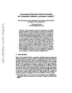
3.3. Examples As a first example consider the 1-bit memory shown in Figure 2. If the signal we (write enable) is set to 1, the flipflop is updated with the value of the input din. Otherwise it keeps its value. To verify an implementation of this simple memory cell, a PSL (property specification language [1]) property has been specified (see Figure 3). It states that whenever we is set, the value of din can be seen at the output dout one cycle later. The property holds. It can now be checked whether the behavior of the memory cell is covered by this property. Therefore, a coverage property is generated (see Figure 4). In line 2 a special command enclosed in a comment instructs the verification tool to insert a multiplexor at signal dout with a select signal named sel. In the antecedent of the coverage property it is assumed that property WRITE holds (line 4)1 . Furthermore it is assumed that the sel signal is set to 1 in the first cycle, i.e. the original value of dout is routed to the output. Under these assumptions it has to hold that the select signal is 1 in the next cycle (line 7). As a result, the coverage property fails and a counterexample is generated which is shown in Figure 5. The case that has not been covered can be deduced from the trace. 1 This is expressed in PSL using the c-like ?-operator for an if-then-else construct, i.e. the property A ⇒ C is transformed to A ? C : 1 due to syntactical restrictions of our PSL parser.

0

1

2

din we FF dout dout_orig sel

1 2 3 4 5 6 7 8 9 10 11 12

Figure 5. Counter-example for coverage of the memory cell. 1 2 3 4 5 6

p r o p e r t y NO CHANGE = always ( we == 0 ) −> ( n e x t ( d o u t ) == d o u t );

Figure 6. Additional property for the 1-bit memory. din

FF0

FF1

FF2

dout

Figure 7. FIFO. Apparently it has not been specified how the memory cell behaves if the signal we is set to 0. As a consequence the sel signal can be set to 0 in the second cycle without violating the property WRITE. After adding an appropriate property like in Figure 6, the output is fully covered. The additional property NO CHANGE states that the output remains unchanged as long as the write enable signal is set to 0. As a second example we consider a FIFO of depth 3 that filters some value, i.e. the output is set to 0 if the last three inputs are 1. See Figure 7 for the implementation of the FIFO. The two basic properties for the FIFO are shown in Figure 8. In the first property the regular shifting of the FIFO is proven if the content of the FIFO is different from three times 1. The second property proves the filtering of the FIFO. Note that the comma operator is used here for concatenation of the three values of the flip flops to one memory word. Both properties hold. We check if the output dout of the FIFO is covered with the coverage property given in Figure 9. Again the multiplexor is inserted with the special command in line 2. For the FIFO and the given properties tmax is 3. Thus, the property SHIFT is assumed without shifting because o is already constrained at time point tmax . However, the property FILT has to be shifted such that the output dout is constrained

p r o p e r t y SHIFT = always ( n e x t [ 3 ] ( ( FF0 , FF1 , FF2 ) ! = ” 111 ” ) ) −> ( n e x t [ 3 ] ( d o u t ) == d i n ); p r o p e r t y FILT = always ( ( FF0 , FF1 , FF2 ) == ” 111 ” ) −> ( d o u t == 0 );

Figure 8. PSL property for the FIFO. 1 2 3 4 5 6 7 8 9 10 11 12 13 14 15 16

p r o p e r t y COV = / / @insertMuxForSignal : dout s e l always ( / / SHIFT ( n e x t [ 3 ] ( ( FF0 , FF1 , FF2 ) ! = ” 111 ” ) ? ( n e x t [ 3 ] ( d o u t ) == d i n ) : 1 ) && / / FILT p r o p e r t y was s h i f t e d next a [ 0 . . 3 ] ( ( ( ( FF0 , FF1 , FF2 ) == ” 111 ” ) ? ( d o u t == 0 ) : 1 ) ) && n e x t a [ 0 . . 2 ] ( s e l == 1 ) ) −> ( n e x t [ 3 ] ( s e l == 1 ) );

Figure 9. Coverage property for the FIFO output. in this property at time point tmax (shifting is done using the next a operator which constraints the following expression to hold at every time point during the specified interval; see line 9). The last expression in the antecedent forces the select input to be 1 up to time point 2 (see line 13). In the consequent we want to show that the select input is 1 at time point tmax = 3. The verification tool reports that the coverage property holds and therefore the FIFO output is covered by the given two properties. Based on these two examples the generation of the coverage property for a simple and a more complex property with respect to several time points have been shown. In the following our approach is studied on a RISC CPU.

4. Experimental Results In this section the application of our method is exemplified through a RISC CPU. First, the basic data of the CPU is briefly reviewed. Then it is shown how the coverage analysis can be carried out. Finally we discuss in which ways the coverage gap can be closed.

4.1. RISC CPU The CPU has been designed as a Harvard architecture. The data width of the program memory and the data memory is 16 bit. The size of the program memory is 4 KByte and the size of the data memory is 128 KByte. The length of an instruction is 16 bit. Due to page limitation we only briefly describe the five different classes of instructions in the following: 6 load/store instructions, 8 arithmetic instructions, 8 logic instructions, 5 jump instructions and 5 other instructions. Since the program counter of the CPU will be used in the following sections, we give some more details on this hardware module. In order to address the 2048 entries of the program memory the PC has an 11 bit register which holds the address of the current instruction. Output pcout holds this address. pcinc outputs the address increased by one. An address can be loaded into the PC via the input din, if the signal le (load enable) is set to 1. Using the reset signal, the PC can be reset to 0. On every positive edge of the clock signal the current address is increased if the signal en (enable) is set to 1.

4.2. Formal Verification To verify the functional behavior of the RISC CPU, a number of PSL properties have been formulated. Figure 10 shows the properties concerning the PC, in particular the ones for the output pcout. Property RESET checks the correct reset behavior. Property INC states that the PC is increased if no reset occurs, no new address is loaded and if the enable signal is set to 1, unless the end of the address space is reached. Finally, property LOAD checks that a new address can be loaded into the PC if le and en are set to 1. All properties have been successfully verified using BMC [14].

p r o p e r t y RESET = always ( r e s e t == 1 ) −> ( next [ 1 ] ( p c o u t == 0 && p c i n c == 1 ) ); p r o p e r t y INC = always ( r e s e t == 0 && l e == 0 && pc < 2047 ) −> ( next [ 1 ] ( ( prev [ 1 ] ( en ) == 1 ) ? ( p c o u t == prev [ 1 ] ( pc ) + 1 ) : ( p c o u t == prev [ 1 ] ( pc ) ) ) ); p r o p e r t y LOAD = always ( r e s e t == 0 && l e == 1 ) −> ( next [ 1 ] ( ( prev [ 1 ] ( en ) == 1 ) ? ( p c o u t == prev [ 1 ] ( d i n ) ) : ( p c o u t == prev [ 1 ] ( pc ) ) ) );

1 2 3 4 5 6 7 8 9 10 11 12 13 14 15 16 17 18 19 20 21 22 23 24 25 26 27 28

Figure 10. PSL properties for the program counter. 0

1

2

en le reset select

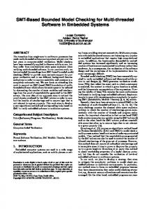
4.3. Coverage Analysis The properties described above are supposed to cover all possible scenarios in the behavior of the PC. The coverage property for the output pcout is generated from the three properties RESET, INC and LOAD, as described in Section 3.2. It appears that the coverage property fails. Figure 11 shows a counter-example that has been generated by the verification tool. From the trace it can be concluded which scenario has not been specified by the properties discussed in Section 4.2. As can be seen in the figure, none of the properties covers the case that the PC is enabled, there is no reset or load, and the PC points to the end of the address space. At the same time, the trace gives information on the actual behavior of the circuit in the unregarded case. Signal pcout orig gives the original value of pcout. Obviously, the PC starts over at address 0 when it exceeds the highest possible address.

pcout_orig pcout_orig_not pcout

2047

0

0

2047

2047

2047

Figure 11. Counter-example for program counter coverage. Before closing this gap we present the results of the coverage analysis phase in Table 1. In the same way every hardware block of the CPU has been checked based on the coverage approach. The first column of Table 1 gives the name of the module. In the second column the number of generated coverage properties is provided. The column cov reports whether all outputs were covered. If not, the last column provides the solution. As can be seen we found three gaps in total. The details on closing these gaps and gaps in general are discussed in the next section.

Table 1. Results of coverage analysis. module # p cov solution ALU 17 no added property program memory 2 yes data memory 2 yes register bank 4 yes program counter 3 no excluded states stack pointer 3 no excluded states control unit 19 no added 2 properties, excluded states

4.4. Closing the Gap If a gap has been found using the presented coverage approach, there are different ways how to deal with it. It is possible that the verification engineer has in fact forgotten to check a certain scenario. In this case the properties have to be completed until coverage is achieved. For the RISC CPU we found that the properties for the ALU did not specify the value of the carry bit in case of a logical operation. Therefore, we added an according property. In the same way we had to add two properties in order to cover the behavior of the control unit in terms of our approach (see Table 1). For example it was not properly specified how the I/O interface behaves during a reset. It is also possible that some scenarios have been left out intentionally, possibly because the specification itself is incomplete. In this case the assumptions of the coverage property can be extended to exclude these states explicitly. Referring to the example in Section 4.3, the specification did not define the behavior of the PC at the end of the address space. It is left to the programmer of the CPU to avoid an address overflow. This is expressed by excluding the state 2047 in the coverage property. Thereby, the program counter was fully covered. In Table 1 this procedure is denoted as ”excluded states”. As can be seen in the table, in three of the modules there have been gaps that were considered harmless. For example one of the gaps in the control unit was related to inactive parts of the data path. In these cases the coverage was completed by excluding the respective states directly in the coverage properties. In total by the presented coverage approach we found three coverage gaps. Following the described steps we achieved 100% coverage.

5. Conclusions In this paper we have presented a pragmatic coverage approach for bounded model checking. The approach generates for each considered output a coverage property after a slight modification of the original design using multiplexors. Thus, the approach can be easily integrated in a standard verification tool. Besides the coverage result itself the main strength of the presented coverage approach is that uncovered scenarios are generated automatically in

form of counter-examples. Closing the coverage gap can be performed by the verification engineer stepwise by analyzing the counter-examples. This clearly improves design understanding.

References [1] Accellera Property Specification Language Reference Manual, version 1.1. http://www.pslsugar.org, 2005. [2] M. Ali, A. Veneris, S. Safarpour, R. Drechsler, A. Smith, and M.S.Abadir. Debugging sequential circuits using Boolean satisfiability. In Int’l Conf. on CAD, pages 204–209, 2004. [3] N. Amla, X. Du, A. Kuehlmann, R. P. Kurshan, and K. L. McMillan. An analysis of SAT-based model checking techniques in an industrial environment. In Correct Hardware Design and Verification Methods (CHARME), pages 254– 268, 2005. [4] A. Biere, A. Cimatti, E. Clarke, and Y. Zhu. Symbolic model checking without BDDs. In Tools and Algorithms for the Construction and Analysis of Systems, volume 1579 of LNCS, pages 193–207. Springer Verlag, 1999. [5] R. Bryant. Graph-based algorithms for Boolean function manipulation. IEEE Trans. on Comp., 35(8):677–691, 1986. [6] R. Bryant. Binary decision diagrams and beyond: Enabling techniques for formal verification. In Int’l Conf. on CAD, pages 236–243, 1995. [7] J. Burch, E. Clarke, K. McMillan, and D. Dill. Sequential circuit verification using symbolic model checking. In Design Automation Conf., pages 46–51, 1990. [8] H. Chockler, O. Kupferman, and M. Vardi. Coverage metrics for temporal logic model checking. In Tools and algorithms for the construction and analysis of systems, number 2031 in Lecture Notes in Computer Science, pages 528 – 542, 2001. [9] H. Chockler, O. Kupferman, and M. Y. Vardi. Coverage metrics for formal verification. In Correct Hardware Design and Verification Methods (CHARME), pages 111–125, 2003. [10] K. Claessen. A coverage analysis for safety property lists. Presentation at Workshop on Designing Correct Circuits (DCC), 2006. [11] E. M. Clarke, O. Grumberg, and A. Peled. Model Checking. MIT Press, 1999. [12] G. Fey and R. Drechsler. Improving simulation-based verification by means of formal methods. In ASP Design Automation Conf., pages 640–643, 2004. [13] G. Fey and R. Drechsler. SAT-based calculation of source code coverage for BMC. In GI/ITG/GMM-Workshop, 2006. [14] D. Große, U. K¨uhne, and R. Drechsler. Hw/sw coverification of embedded systems using bounded model checking. In Great Lakes Symp. VLSI, pages 43–48, 2006. [15] Y. V. Hoskote, T. Kam, P. Ho, and X. Zhao. Coverage estimation for symbolic model checking. In Design Automation Conf., pages 300–305, 1999. [16] N. Jayakumar, M. Purandare, and F. Somenzi. Dos and don’ts of ctl state coverage estimation. In Design Automation Conf., pages 292–295, 2003. [17] S. Katz and O. Grumberg. Have I written enough properties - a method of comparison between specification and implementation. In Correct Hardware Design and Verification Methods (CHARME), pages 280–297, 1999. [18] K. Winkelmann, H.-J. Trylus, D. Stoffel, and G. Fey. Costefficient block verification for a UMTS up-link chip-rate coprocessor. In Design, Automation and Test in Europe, volume 1, pages 162–167, 2004.