parallel application workloads that run on these HPC resources can be difficult to understand without detailed workload energy consumption and power profiles.
This paper appears in the 2017 IGSC Track on Contemporary Issues on Sustainable Computing
Evaluating Energy and Power Profiling Techniques for HPC Workloads Ryan E. Grant, James H. Laros III, Michael Levenhagen, Stephen L. Olivier, Kevin Pedretti, Lee Ward, Andrew J. Younge Center for Computing Research, Sandia National Laboratories* P.O. Box 5800, MS-1319, Albuquerque, NM 87185-1319 Email: {regrant,jhlaros,mjleven,slolivi,ktpedre,lee,ajyoung}@sandia.gov
Abstract—Advanced power measurement capabilities are becoming available on large scale High Performance Computing (HPC) deployments. There exist several approaches to providing power measurements today, primarily through in-band (e.g. RAPL) and out-of-band measurements (e.g. power meters). Both types of measurement can be augmented with application-level profiling, however it can be difficult to assess the type and detail of measurement needed to obtain insight from the application power profile. This paper presents a taxonomy for classifying power profiling techniques on modern HPC platforms. Three HPC mini-applications are analyzed across three production HPC systems to examine the level of detail, scope, and complexity of these power profiles. We demonstrate that a combination of out-of-band measurement with in-band application region profiling can provide an accurate, detailed view of power usage without introducing overhead. This work also provides a set of recommendations for how to best profile HPC workloads.
I. I NTRODUCTION As extreme-scale High Performance Computing (HPC) platforms grow, so do the power requirements to operate such expansive computing systems. Current leadership-class HPC facilities are now built with power envelopes on the order of Megawatts, with current US Department of Energy (DOE) Exascale projections in the 20-40MW range. Practical power delivery issues at the facility level mean that managing power consumption of these systems is important. However, power measurement capabilities on large scale HPC systems have historically been very limited or non-existent, limiting the ability to understand and manage large system power usage. Furthermore, the power consumption of bulk synchronous parallel application workloads that run on these HPC resources can be difficult to understand without detailed workload energy consumption and power profiles. Emerging systems are now capable of managing power measurements of some individual components, whole nodes and even the entire system. One class of methods are in-band measurement techniques, including reading CPU counters like *Sandia National Laboratories is a multimission laboratory managed and operated by National Technology and Engineering Solutions of Sandia, LLC., a wholly owned subsidiary of Honeywell International, Inc., for the U.S. Department of Energy’s National Nuclear Security Administration under contract DE-NA0003525.
Intel’s Running Average Power Limit (RAPL). In contrast, outof-band measurements from dedicated hardware are capable of measuring and reporting data without the intervention or involvement of the compute resources on the board. In addition to the mechanisms used to gather power consumption data, in-line code instrumentation methods can be used to directly annotate application code to identify code regions of interest and correlate them with power measurements. Power measurement and characterization of HPC applications is a well established field. We will show that a compilation of techniques can lead to insight that was not otherwise possible. While the individual techniques described herein have been used and studied previously, we demonstrate a combination of techniques now available on cutting edge systems provides greater profiling detail than any single technique, leading to better insight. This work presents a detailed power profiling study of in-band, out-of-band, and application profiling not collectively examined in previous work. This paper makes the following contributions: •
•
•
•
We present a taxonomy for classifying the power profiling techniques available on modern HPC platforms. This framework is useful to HPC practitioners to understand and discuss power profiling studies of HPC workloads. Through analysis of three example mini-applications, we demonstrate how power profiling accuracy and overhead differ among the available techniques on multiple recent platforms. In particular, we show how the common practice of relying on only aggregate job-wide information such as total energy consumed can be misleading. We demonstrate a unique combination of out-of-band power profiling together with in-band application region profiling, which produces an accurate view of application power usage behavior with negligible runtime performance overhead on production HPC platforms. Finally, we provide a set of recommendations and best practices for performing power profiling of HPC workloads, taking into account our experience.
The rest of the paper is as follows. First, it provides some background on the power profiling capabilities that exist on HPC systems. Next, it defines our detailed taxonomy of mea-
c 978-1-5386-3470-7/17/$31.00 2017 IEEE
surement and application evaluation strategies to guide readers through the complexity, advantages, and trade-offs of different power profiling techniques. Then, three mini-applications are evaluated across three different HPC systems to illustrate the measurement taxonomy by sampling simple aggregate runtime data, expanding detail with application profiling, and then correlating in-band and out-of-band data measurements using a P-state sweep and CPU architecture comparisons as case studies. The paper concludes with recommendations based on the insight desired, the target platform’s capabilities, and the amount of effort required. II. BACKGROUND Power measurement of system components is a topic that has been studied for many years. Accurate power measurements are essential when energy budgets are regulated and finite, such as in mobile devices. Energy usage is important in real-time applications to identify opportunities to reduce energy usage while satisfying required deadlines. Commercial services such as cloud providers focus on overall system efficiency for cost optimization. Power usage is also of interest to sites hosting HPC platforms, as such sites must meet statutory regulations governing energy efficiency and seek to minimize electricity costs. However, US DOE HPC facilities are often more concerned with limitations that constrain the amount of power that can be provided to a given platform. Approaches to power measurement are varied, and provide different types and rates of data. Out-of-band measurement is the easiest approach to understand. It uses equipment external to the compute resource to measure power consumption without perturbing computational performance. Classic examples of out-of-band measurement include devices like WattsUp! [1], WattProf [2], PowerInsight [3], and integrated devices like IBM’s power measurement capabilities [4]. Out-of-band measurements avoid perturbing the ongoing computation, but they may not provide easily accessible information to the running processes. Since these devices are necessarily not part of the CPU, they must be interrogated over external device buses for data instead. Historically, simple out-of-band measurement techniques have had relatively low sampling rates, however new integrated designs have greatly improved sampling rate. In-band measurement uses device-level integrated measurement capabilities, such as Intel’s Running Average Power Limit (RAPL), or AMD’s Advanced Power Management (APM). They provide real or estimated measurements of energy consumption through device-level interfaces. RAPL and APM use CPU counters to express energy usage, and can provide separate core, package and DRAM measurements. Inband measurements require active participation of the compute cores in a system to gather data on a regular basis. Therefore, point-in-time samples require frequent intervention to record the values in counters on the device. This corresponds to a read of a CPU register on both Intel’s and AMD’s solutions. If only total energy consumption of the whole application is needed, rather than point-in-time samples, then in-band measurement can have very little impact on computational performance. Point in time samples require several reads per second if the device’s maximum sampling rate is used.
In-band measurement through CPU counters can often provide both CPU and memory subsystem energy measurement [5], [6]. This is not always possible with out-of-band measurement, depending on where the external measurement hardware is placed and its capabilities. Out-of-band measurement can capture whole node energy profiles more easily, while this is generally not possible for in-band measurement that relies on CPU counters. Whole node energy can be useful when other components such as network or motherboard chip set consume a large amount of the power budget for a node. Application instrumentation and profiling can take multiple forms. Timestamping is a common practice amongst application developers to understand the performance characteristics of their code. Other more in depth profiling techniques and tools such as Intel’s Vtune [7] or Cray’s CrayPat [8] allow deeper inspection into program behavior through call-graph traces and CPU performance monitoring counter data. The Power API [9] can provide a portable solution to application level power measurement when application region hints are integrated with power measurement through the framework. III. TAXONOMY OF P OWER M EASUREMENT Modern large-scale HPC platforms have incorporated several forms of power measurement and energy accounting that expand the possibilities of gathering key data. However, it is often difficult to know where to start or, in many cases, difficult to access the information that is available. In this section, we describe a framework for understanding these capabilities and discuss the potential insight they can provide. A. Level 1: Job-wide Aggregate Information Many platforms track coarse-grained power and energy usage continuously, such as total energy usage by each application executed. It may be broken down by component, e.g., separate CPU and memory energy values, but the information is usually aggregated over an entire application run rather than point-in-time samples or per-node information. The information collected may be available to users in a post-job report. Job-wide energy information helps to understand how energy-to-solution changes for different application optimizations, algorithm choices, or run configurations. It can also be useful for performance tuning. High power usage levels (e.g., as a percent of the peak available budget) often indicate a well tuned application, whereas low power usage levels may indicate room for further optimization. A downside to this technique is that it only provides insight into energy usage behavior in aggregate, not the varying rates of energy consumption throughout an application’s execution. B. Level 2: Periodic Sampling Finer-grained detail is provided by periodically sampling power levels and energy usage over time. This is often how level 1 information is derived. Sampling may be implemented in-band or out-of band. With in-band, compute node resources are used to perform the sampling, reducing the resources available for application execution. With out-of-band, the
platform’s control system infrastructure is used to implement the sampling without using compute node resources. Many platforms store a short time window of power and energy samples in a database for use by administrators and workload managers. The information may be accessible to users, but obtaining access often requires administrator action. This information can be used to plot power usage versus time. It is often possible to identify different application regions by looking for changes in power level. Activities such as idle periods, network polling, and I/O phases can sometimes be identified and used to diagnose load imbalance issues within an application. A downside to this technique is the potentially large volume of point-in-time sample information that must be retained and the difficulty of analyzing it. A concern with in-band sampling is the performance degradation of the application itself due to frequent interruption of the CPU to read the hardware counters. This interruption not only pauses compute tasks but can also pollute the CPU cache, which may also impact total energy consumption and effect time measurements. While it may seem a small impact overall, previous experience with OS system noise shows that even minor interruptions can induce larger slowdowns when processes must synchronize across the application [10]. C. Level 3: Application Instrumentation While the first two levels treat the application as a black box, or as a gray box when application knowledge is used to interpret the recorded information, white box analysis is useful to understand an application’s internal behavior at a finer level of detail. One can modify an application to instrument code regions of interest. The instrumentation points can then be used to record in-band power and energy samples during execution. This information can be analyzed to characterize each instrumented region’s power and energy usage behavior. The potential downsides of this technique are that it requires application modifications and may reduce performance due to instrumentation overhead. The effort needed to instrument an application can be reduced by using automated tools or amortized by leveraging the instrumentation points for other purposes, such as for input to an introspective runtime system. Overheads from application instrumentation depend greatly on two different factors. The first is the complexity of the instrumentation in terms of the data that must be gathered. Some low overhead methods simply use time stamp and region tuples [11]. Timing has been used for a long time in HPC applications, especially using MPI [12] timing functions to instrument code regions of interest. Some instrumentation also incorporates information from sources like performance monitoring counters [13], which can even be used to estimate power consumption without hardware measurement support [14]. The second factor that impacts overhead is sampling frequency. Even with lightweight sampling, for short regions the timestamp can be called so often that it begins to impact performance. If a region is only 1000 cycles with 50 cycles to read and record the data then 5% overhead is incurred. Our evaluation uses regions long enough to amortize overheads for simple sampling like timestamp-region tuples. However,
the cost must be taken into account when instrumenting applications to avoid high levels of overhead. D. Level 4: Multi-Level Correlation Finally, information gathered from previous levels can be cross-correlated and used to derive information that is not otherwise available, or would be too costly to obtain using a single level in isolation. For example, if the overhead of application instrumentation (level 3) is too high, power measurement at instrumentation points could be disabled with only timestamps kept. The timestamps could then be correlated with out-of-band periodic power samples (level 2) to obtain similar insight with less application overhead. As another example, if a particular application run experienced an unexplained performance degradation (e.g., a “slow run”), level 1 information could be inspected to look for anomalous power or energy usage behavior. To probe deeper, the level 1 job start and end timestamps could then be used to generate a power versus time plot from level 2 information. The plot may reveal clues to the reason for the slowdown, such as a concentrated idle period (e.g., a system I/O issue or network quiesce event). Aligning application instrumentation timestamps with inband and out-of-band periodic sampling measurements can be difficult. In-band measurements are typically the easier of the two to align as they can use the same timestamp as the application instrumentation (region timestamping). In this approach one can use system timestamps and reasonably expect them to line up with relative ease. Out-of-band measurements can be much more complex to align with region timestamps. Because the measurement hardware is separate and distinct from the CPU, absolute timestamps from measurements, applications timestamps, and hardware power samples are needed. To align these time samples, the user must find the minimum timestamp for both the application region profile output and the out-ofband measurements. Using this minimum, one can establish an offset for the individual timestamps and based on a common start point t = 0. From there timestamps can be lined up and produce useful data for analysis. IV. E XPERIMENTAL R ESULTS A. Test Platforms We evaluated power/energy measurement techniques on three different Cray platforms. One platform, Volta, was a standalone Cray XC30 testbed system with dual socket IvyBridge E5-2695v2 CPUs and 64GB RAM and a max node power draw of 350W. The IvyBridge CPU has a frequency range of 1.2 - 2.4 Ghz with a turbo frequency of 3.2 Ghz. The other two systems are different implementations of a Cray XC40 system, the first comprising a traditional dual socket Haswell E5-2698v3 CPUs and 128GB RAM, and the second consisting of a single socket Knights Landing (KNL) Xeon Phi 7260 with 96GB RAM and 16GB MCDRAM. The Haswell XC40 has a max power draw of 415W per node and a CPU frequency range of 1.2 - 2.3 Ghz with max turbo of 3.6 Ghz, whereas the KNL Phi has a max power draw of 345W per node and a frequency range of 1.0 - 1.4 Ghz, with 1.6 Ghz turbo frequency. All three systems utilize the same
Cray Aries Interconnect. Here, the XC40 systems represent a small system that is identical to the hardware and software of the Trinity supercomputer, currently the tenth fastest computer on the Top500 list [15]. The three test platforms provide similar power measurement capabilities. Level 1 information is provided by Cray’s RUR (Resource Utilization Reporting) tool [16], which records various aggregate statistics about each job, including start time, end time, and total energy consumed. Level 2 information is provided by Cray’s out-of-band power monitoring infrastructure and Power Management Database (PMDB). Per-node power is sampled at 5 Hz and stored in the PMDB PostgresSQL database, with a rolling 4 hour window of samples kept for each system. Each compute node contains a power measurement device with accuracy of +/- 3% that is internally sampled at a rate higher than 5 Hz. For the Trinity platforms, each 5 Hz power sample is the average of the internal samples since the previous 5 Hz sample. The XC30 (Volta) runs an older Cray management software release that does not perform this averaging, so the 5 Hz value recorded represents the most recent internal sample available. Level 3 application instrumentation for this study uses the KokkosP runtime profiling interface [17], part of the Kokkos C++ performance portability library1 . KokkosP provides lowoverhead profiling and instrumentation of applications. We have used KokkosP exclusively to denote application region entry/exit with timestamps, as described later. We also developed a Power API plugin for KokkosP to collect in-band power and energy measurements. Some but not all applications in the study use the Kokkos programming model, demonstrating that the KokkosP lightweight profiling library can be used independently or in conjunction with Kokkos-based code. B. Workloads We used three different miniapplications to conduct our experiments, MiniMD, LULESH and MiniFE. 2 • MiniMD - A molecular dynamics (MD) miniapplication representing the LAMMPS [18] full featured MD simulator. While MiniMD supports only Lennard-Jones (LJ) pair interactions, its behavior is essentially equivalent to LAMMPS for the LJ liquid simulation it performs. 3 • LULESH - An unstructured mesh Lagrangian explicit shock hydrodynamics miniapplication [19], representing DOE hydrodynamics applications, especially ALE3D. 4 • MiniFE - An implicit finite element (FE) conduction simulation using a conjugate gradient (CG) solver on a rectangular shaped problem. To represent a broad class of FE applications, its CG solver is simple and generic [20]. These workloads were run on 32 nodes of each platform using all cores on each node. The same input problem was used across test platforms, enabling cross architecture comparisons. Input problems were chosen by consulting with subject matter experts to determine realistic configurations that would produce high performance across the three platforms studied. 1 https://github.com/kokkos 2 https://github.com/Mantevo/miniMD 3 https://codesign.llnl.gov/lulesh.php 4 https://github.com/Mantevo/miniFE
C. Job-wide Aggregate Information Aggregate counts of total energy consumed or average wattage over a sampling period are obtained using hardware registers that are polled for values only at the beginning and end of an application execution. This is technically in-band as the commands are issued to read the hardware counters from the CPUs executing the simulation code. Reading these counters can be done with negligible overhead, as the code reads the counter before and after the application execution, avoiding any interference while running the simulation. To demonstrate the initial utility of HPC job aggregate information, we look at a common case study where a P-state sweep is performed to try to determine a configuration for the highest performing, the lowest overall power consumption, or the least total energy consumed per Figure of Merit (FOM) 5 . Given 3 architectures and turbo-boost frequencies, we also use the 1.2 GHz frequency results to compare different CPU architecture types at an identical clock speed. Results from this study are shown in Table I. These results demonstrate trends that are predictable: The fastest clock speeds are almost universally the most performant mode of operation for all architectures. The exception is Haswell running MiniFE, where non-turbo max frequency is slightly better than turbo but within the margin of error. In terms of FOM per watt, the results are less straightforward. The Ivy Bridge system should be run in non-turbo highest frequency for power efficiency and performance, but for the Haswell and KNL systems the ideal frequency varies based on the architecture and application. The KNL and Xeon core architectures are vastly different x86 implementations. The results show that the many Intel Atom-based cores in the KNL architecture are better for both MiniMD and MiniFE. For the memory-intensive LULESH code, however, the high bandwidth, low latency memory subsystem in the Xeon allows it to slightly outperform KNL. Unfortunately, this case study also illustrates the limitations of aggregate job information. First, this aggregated data cannot tell us which particular phase of an application is of concern or how energy is consumed throughout execution. Other techniques are necessary to answer these questions. Perhaps more alarmingly, the total job energy consumption may lead us to false conclusions about optimizing FOM per watt. With MiniFE, the Trinity Haswell portion shows 1.2Ghz to be the best FOM per watt. However, as we find later when application code regions are instrumented, MiniFE’s FOM is based on a single region that is a small portion of the total runtime, effectively leading to a false conclusion regarding selecting an optimal P-state FOM per Watt. D. Application Instrumentation Compared to simplistic aggregate job data, application profiling requires significantly more effort and knowledge of the applications under study than aggregate counter or out-ofband power measurement. It can yield more insight into the power and energy characteristics of applications. However, the detail and frequency at which application instrumentation is implemented can have cascading impacts and considerations. 5 FOM
is a measure of application performance, e.g., elements/second.
TABLE I P OWER AND E NERGY E FFICIENCY C ALCULATED FROM C RAY RUR AGGREGATE I NFORMATION Figure of Merit Per Node
Average Watts Per Node
Figure of Merit Per Watt
Volta Ivy Bridge
Trinity Haswell
Trinity Phi KNL
Volta Ivy Bridge
Trinity Haswell
Trinity Phi KNL
Volta Ivy Bridge
Trinity Haswell
Trinity Phi KNL
MiniMD
Turbo No Turbo 1.2 GHz
2.08e7 1.84e7 9.45e6
3.01e7 2.56e7 1.39e7
5.92e7 5.66e7 4.93e7
269 213 138
334 236 142
246 228 194
7.73e4 8.64e4 6.85e4
9.01e4 1.08e5 9.79e4
2.41e5 2.48e5 2.54e5
LULESH
Turbo No Turbo 1.2 GHz
1.36e4 1.24e4 6.75e3
1.85e4 1.75e4 1.09e4
1.51e4 1.43e4 1.25e4
291 236 156
346 295 175
218 208 180
46.7 52.5 43.3
53.5 59.3 62.3
69.3 68.8 69.4
MiniFE
Turbo No Turbo 1.2 GHz
1.24e4 1.23e4 8.37e3
1.42e4 1.43e4 1.41e4
3.00e4 2.93e4 2.76e4
185 145 104
212 152 104
138 133 127
67.0 84.8 80.5
67.0 94.1 136
217 220 217
For more insight into application behavior we need to understand the phases of the applications themselves. Table II shows the region breakdown for each of the three applications operating with the KNL turbo P-state. The number of occurrences of each region are identical across architectures and only the region timings vary. MiniMD has 5 main regions. Not all of these regions occur in every timestep of the simulation. For example, NeighborBuild is only run every 20 timesteps. However, when it does occur it is a significant portion of the execution time for that timestep. Like MiniMD, LULESH also has 5 regions in its main solve. Regions 2 and 5 are the most significant in terms of time, while region 3 is very short. Like Exchange or Communicate regions for MiniMD, region 3 is very difficult to profile. This is because the region is so short that measurement may not be possible inside of the region. For MiniFE, we have only instrumented the assembly and CG solves as regions. Since both regions are large, the power profile clearly differentiates these two regions in Figure 1c. TABLE II A PPLICATION P ROFILING R EGION D URATIONS F OR T RINITY KNL
both power/energy readings and timestamps, as well as with only timestamps enabled, are shown in Table III. Our initial investigation for KNL yielded significant overheads of in-band sampling with region profiling for MiniMD and LULESH, ranging form 4-8%, whereas MiniFE in-band sampling was negligible compared to no sampling. These overheads are significant even at a small scale. Given prior knowledge of how asynchronous noise in parallel applications can have cascading effects at a large scale, these overheads could increase when moving to an extreme scale such as the Trinity supercomputer. TABLE III OVERHEAD OF A PPLICATION P ROFILING F OR T RINITY KNL
Count
Mean
SD
MIN
MAX
Exchange CommBorders MiniMD Communicate Force NeighborBuild
1632 1632 30400 32000 1600
0.005 0.010 0.003 0.039 0.600
0.002 0.009 0.003 0.009 0.002
0.003 0.006 0.002 0.036 0.595
0.025 0.085 0.032 0.155 0.624
IntegrateStress HourglassControl LULESH VelocityForNodes LagrangeElements MonotonicQ
25600 25600 25600 25600 25600
0.011 0.039 0.002 0.018 0.031
0.000 0.001 0.000 0.001 0.005
0.010 0.038 0.001 0.017 0.023
0.035 0.067 0.002 0.066 0.063
MiniFE
Assemble CGSolve
32 135.243 5.465 125.582 149.543 32 14.209 0.000 14.208 14.210
Power/energy profiling can be done inline in the application directly through in-band measurement, such as calling the PowerAPI or interfacing with RAPL directly. However, the overhead of in-band measurement can be significant when sampling at high frequency. To quantify the potential overhead of inline application profiling, multiple experiments with
Timestamps Only
MiniMD
Turbo 1.4 GHz 1.2 GHz 1.0 GHz
6.84% 7.49% 7.71% 8.15%
-0.08% -0.08% 0.08% 0.07%
LULESH
Turbo 1.4 GHz 1.2 GHz 1.0 GHz
4.84% 4.94% 5.23% 4.73%
0.24% 0.35% 0.22% -0.08%
MiniFE
Turbo 1.4 GHz 1.2 GHz 1.0 GHz
-1.22% -0.59% -1.50% -1.26%
0.15% -0.95% -1.42% -1.96%
Region Durations (seconds) Region Name
Power + Energy Region Profiling
When we disable profiling and use only timestamping, the performance overheads become essentially non-observable when accounting for normal application runtime variance in measurement. Timestamping is currently the best way to couple application profiling with out-of-band power samples. Since out-of-band samples are detached from the application or compute infrastructure entirely, the use of timestamps within the application becomes the only feasible way to couple out-of-band data. While it requires significant additional effort and synchronized clocks, the result is a near complete lack of perturbation or added overhead due to profiling. E. Out-of-band Periodic Sampling Out-of-band power sampling can provide detailed information about application phases and the impact of varying
clock frequency on the CPU. Continuing with the case study detailed in Table I, we next look at P-states across the KNL system. In Figure 1, the power versus time plots include level 2 power samples taken at 5 Hz for each of the 32 nodes for the respective run, with a solid horizontal line added to visualize the job-wide average power calculated from level 1 information. MiniMD’s out-of-band measurements in Figure 1a show expected behavior in the main solve of the application. The periodic power consumption corresponds with known solver phases, and each P-state shows the expected number of phases. Using a slower CPU frequency lengthens the phases but does not alter any observable power consumption trends. LULESH’s power consumption with varying CPU frequency for the KNL is shown in Figure 1b. Its power consumption is much less periodic than MiniMD but shows similar patterns of lowered power consumption and lengthened runtimes with different P-states. Unlike MiniMD, where phases are obvious in the power consumption graph, LULESH has 5 phases, but all of them are similar in power consumption, even though the time periods of the individual phases are not equal (some are very short, others are longer than average). MiniFE shows multiple different phases throughout execution in Figure 1c. The first long, low-power phase is the assembly phase while the increased power consumption regions are the problem solve (CG). We can observe that power usage throughout the assembly phase is slightly improved by lowering the CPU frequency. However, the difference is not as large as the power savings during the main CG solve region. This will impact the performance per watt of the lower frequency results as the assembly phase is the longest phase. In addition to an analysis of P-states on KNL only, we can also directly compare all three of our platforms with out-of-band measurement. The results for MiniMD, shown in Figure 2, illustrate some differences between the out-of-band measurement techniques across the 3 system platforms. The out-of-band measurement capabilities between these systems are very similar, except that the Ivy Bridge system reports only point-in-time power samples, while the Haswell and KNL systems average results between sampling reading points. This leads to a much less noisy power profile for the newer systems, avoiding spurious data not significant to the analysis of the power consumption of the system. The results can be significant for identifying periodic power behavior in an application. In Figure 2 we observe that the KNL system shows clear periodic behavior that we can relate back to known phases of the application and timesteps in the simulation itself. Such results on the Ivy Bridge system yield a noisy signal, and the periodicity of the underlying code regions was lost. This is not the case when we have intra-sample averaging like on the KNL/Haswell system. While LULESH (not pictured) does not have the same region periodicity, the noise from LULESH running on IvyBridge was even greater, to the point of obscuring useful data. F. Combining Out-of-band Periodic Sampling and Application Instrumentation Region profiling with timestamps and in-band power/energy profiling paired with the collection of out-of-band data allows
(a) MiniMD
(b) LULESH
(c) MiniFE Fig. 1. Out-of-band power sampling for workloads running on Trinity Knights Landing at different CPU frequencies.
Fig. 2. Out-of-band power sampling for MiniMD running on 3 different test platforms.
significantly more insight than any one technique. Specifically, the method of power data paired with profiling may have drastically different resolutions that effect the perceived accuracy of the interpreted results. Looking at MiniMD in Figure 3, the results show an issue of resolution that can be introduced by power/energy profiling only at region entry and exit. The Figure shows that all of the periodic data with timesteps (in black) of the application
Fig. 3. MiniMD correlating out-of-band power sampling with in-band application region profiling.
are not observable in comparison to in-band measurements (in red), which are taken along region boundaries. The outof-band measurements capture this periodic behavior and, when combined with timestamps, application profiling clearly illustrates which regions correspond to the periodic behavior. While the in-band measurement does accurately report the total energy usage, the rate of usage throughout the region is incorrect as it is treated as a uniform power/energy draw. Effectively, this in-band approximation does not match the finegrained out-of-band measurements or the higher frequency periodic behaviors observed. Other studies have validated inband measurements using out-of-band measurement [21], so while in-band measurements are accurate, it is the lack of the resolution with sampling rate that fails to properly illustrate the application’s true power profile. In-band sampling resolution could be increased by interrupting the application to query the energy counters throughout the execution. One could also define finer-grained regions if appropriate for the code under study, however as seen in Table III, doing so would also add overhead and potential perturbation to the application itself. Furthermore, for coursegrained application regions like MiniFE, the assumed behavior throughout the region is very different than the out-of-band sampling throughout the region. This illustrates a key issue with in-band measurement sampling only between regions: the behavior within a region is not guaranteed to be uniform. V. R ELATED W ORK The concept of investigating energy and power consumption of large-scale HPC resources is not a new one. In the literature, most related work has addressed power measurement using solely out-of-band [22]–[24] or in-band [25]–[27] techniques. Some work has also sought to validate in-band measurements using out-of-band measurements at the same time to determine the overall accuracy of the measurements or integrated power model [6]. Previous work has used application instrumentation with power measurements to estimate energy usage to within 10% of actual consumption [14]. Several works have used estimated power values to determine the system energy consumption [28]–[30]. Other work uses power measurements to illustrate methods for operating power constrained systems [31], [32]. Several power estimation frameworks/simulators exist as well such as WATTCH [33], and SST [34]. However, these simulators rely on estimations of energy consumption
and therefore have high margins of error, particularly for architectures that are not the explicit target of the simulation. APIs have addressed the topic of gathering power and energy data from systems including the Power API [35], Redfish [36], CapMC [37] and AMESTER [38]. Previous work has been limited by the measurement capabilities available on extreme-scale HPC platforms used. For example, Leon et al. [11] used out-of-band measurement and application region marking. Additional work used in-line performance measurement counters (not power counters) to better understand the behavior of individual regions [39]. However, this work did not explore the capabilities nor trade-offs of in-band measurement, and used only traditional multicore CPUs but on a variety of architectures. The work described herein is the first known to address both in-band and out-ofband measurement techniques together on the same hardware and coupled with application profiling for each measurement. Furthermore, this work also contributes a detailed taxonomy to detail how, when, and why HPC application developers can accurately evaluate power consumption. VI. R ECOMMENDATIONS AND D ISCUSSION The key lessons learned from our study can help to guide HPC application profiling for measuring power and energy. One must first decide what level scope is necessary when conducting power profiling. The taxonomy given in Section III assists in determining the level of detail desired, the amount of data available, and the amount of effort required. If only total energy usage or average power for an application are needed but not phase data or periodic consumption rates, aggregate data collection is the best initial option. This is also the first approach to use when detailed application information is not available, such as in-depth knowledge of code regions. Aggregate data has low overhead and requires less storage space and analysis time than the other studied measurement techniques. If application code knowledge is limited, out-of-band data collection or timed in-band periodic counter polling are the best next options. Out-of-band data is the preferred collection method but is often not available since it requires specialized out-of-band hardware like that of the Cray platforms. Moreover, out-of-band data may be available only to administrators, an active policy issue to be resolved at HPC facilities. Time-averaging of samples, if supported in the measurement system, is helpful to discover trends in the application. Phases are more easily discernible if adjacent regions of code do not have similar power profiles. If detailed information on application code regions is necessary and sufficient knowledge of the application is given, then in-line application profiling should follow. Application profiling can be aligned to in-band data through measurement tools like RAPL to sample values surrounding code regions. However, in-band application instrumentation may significantly perturb performance, especially for short regions. Therefore, the best form of measurement for the most in depth understanding is to combine code regions with timestamps and correlate with out-of-band measurements. This method provides low-overhead, fine-grained data over the entire execution
to enable useful observations that would not be visible otherwise. However, this approach requires the greatest amount of effort and knowledge of both the system and application, as well as specialized out-of-band hardware support that is still not yet commonplace. Automating this process is difficult, and the proprietary nature of out-of-band hardware can be limiting. This situation motivates standardization efforts, such as the Power API [9], that can provide a common interface for both application instrumentation timings and out-of-band data. In conclusion, we have demonstrated that no single contemporary measurement technique is sufficient to gather power measurements for all HPC use cases. Instead, the measurement taxonomy introduced in this paper can be applied to determine the appropriate level of detail and effort, as demonstrated by our thorough investigation of multiple proxy HPC applications across multiple production platforms using both in-band and out-of-band data. In particular, we that show that the combination of application region profiling and out-of-band power measurement provides an accurate view of application power profiles with negligible overhead. Our recommendations provide actionable guidance for HPC application profiling to better understand power and energy usage on HPC systems. R EFERENCES [1] Electronic Educational Devices, “Watts up PRO,” 2009. [2] M. Rashti, G. Sabin, D. Vansickle, and B. Norris, “WattProf: A flexible platform for fine-grained HPC power profiling,” in 2015 IEEE Intl. Conference on Cluster Computing (CLUSTER). IEEE, 2015, pp. 698– 705. [3] J. H. Laros, P. Pokorny, and D. DeBonis, “PowerInsight - a commodity power measurement capability,” in 2013 Intl. Green Computing Conference (IGCC). IEEE, 2013, pp. 1–6. [4] R. Bertran, Y. Sugawara, H. M. Jacobson, A. Buyuktosunoglu, and P. Bose, “Application-level power and performance characterization and optimization on IBM Blue Gene/Q systems,” IBM Journal of Research and Development, vol. 57, no. 1/2, pp. 4–1, 2013. [5] AMD, “BIOS and kernel developer’s guide (BKDG) for AMD family 15h models 00h-0Fh processors,” January 2013. [6] H. David, E. Gorbatov, U. R. Hanebutte, R. Khanna, and C. Le, “RAPL: memory power estimation and capping,” in ACM/IEEE Intl. Symposium on Low-Power Electronics and Design (ISLPED). IEEE, 2010, pp. 189–194. [7] J. Reinders, Vtune performance analyzer essentials: Measurement and tuning techniques for software developers, 2005. [8] S. Kaufmann and B. Homer, “Craypat-cray x1 performance analysis tool,” Cray User Group (May 2003), 2003. [9] R. E. Grant, M. Levenhagen, S. L. Olivier, D. DeBonis, K. T. Pedretti, and J. H. Laros III, “Standardizing power monitoring and control at exascale,” Computer, vol. 49, no. 10, pp. 38–46, 2016. [10] K. B. Ferreira, P. Bridges, and R. Brightwell, “Characterizing application sensitivity to os interference using kernel-level noise injection,” in International Conference for High Performance Computing, Networking, Storage and Analysis. IEEE, 2008, pp. 1–12. [11] E. A. Le´on, I. Karlin, and R. E. Grant, “Optimizing explicit hydrodynamics for power, energy, and performance,” in IEEE Intl. Conference on Cluster Computing (CLUSTER). IEEE, 2015, pp. 11–21. [12] MPI Forum, “MPI: A Message-Passing Interface Standard. Version 3.1,” June 2015. [13] B. Sprunt, “The basics of performance-monitoring hardware,” IEEE Micro, vol. 22, no. 4, pp. 64–71, 2002. [14] R. Joseph and M. Martonosi, “Run-time power estimation in high performance microprocessors,” in Proc. of the 2001 Intl. Symposium on Low power electronics and design. ACM, 2001, pp. 135–140. [15] H. Meuer, E. Strohmaier, J. Dongarra, H. Simon, and M. Meuer, “Top500 supercomputing sites,” 2017. [Online]. Available: http: //www.top500.org/ [16] A. Barry, “Resource utilization reporting,” in Proc. Cray Users’ Group Technical Conference (CUG), 2013.
[17] S. D. Hammond, C. R. Trott, H. C. Edwards, and N. Ellingwood, “KokkosP: Runtime hooks for portable performance analysis,” Sandia National Laboratories, Tech. Rep. SAND2016-3679C, 2016. [18] S. Plimpton, “Fast parallel algorithms for short-range molecular dynamics,” J. Comput. Phys., vol. 117, no. 1, pp. 1–19, Mar. 1995. [19] I. Karlin, J. Keasler, and R. Neely, “LULESH 2.0 updates and changes,” Lawrence Livermore National Laboratory, Tech. Rep. LLNLTR-641973, 2013. [20] M. A. Heroux, D. W. Doerfler, P. S. Crozier, J. M. Willenbring, H. C. Edwards, A. Williams, M. Rajan, E. R. Keiter, H. K. Thornquist, and R. W. Numrich, “Improving performance via mini-applications,” Sandia National Laboratories, Tech. Rep. SAND2009-5574, 2009. [21] A. Mazouz, B. Pradelle, and W. Jalby, “Statistical validation methodology of CPU power probes,” in European Conference on Parallel Processing. Springer, 2014, pp. 487–498. [22] A. Tiwari, M. A. Laurenzano, L. Carrington, and A. Snavely, “Modeling power and energy usage of HPC kernels,” in IEEE 26th Intl. Parallel and Distributed Processing Symposium Workshops & PhD Forum (IPDPSW). IEEE, 2012, pp. 990–998. [23] J. Dongarra, B. Tourancheau, S. Song, R. Ge, X. Feng, and K. W. Cameron, “Energy profiling and analysis of the HPC challenge benchmarks,” The Intl. Journal of High Performance Computing Applications, vol. 23, no. 3, pp. 265–276, 2009. [24] B. Mills, R. E. Grant, K. B. Ferreira, and R. Riesen, “Evaluating energy savings for checkpoint/restart,” in Proc. 1st Intl. Workshop on Energy Efficient Supercomputing. ACM, 2013, p. 6. [25] O. Sarood, A. Langer, L. Kal´e, B. Rountree, and B. De Supinski, “Optimizing power allocation to CPU and memory subsystems in overprovisioned HPC systems,” in IEEE Intl. Conference on Cluster Computing (CLUSTER). IEEE, 2013, pp. 1–8. [26] M. Hahnel, B. Dobel, M. Volp, and H. Hartig, “Measuring energy consumption for short code paths using RAPL,” ACM SIGMETRICS Performance Evaluation Review, vol. 40, no. 3, pp. 13–17, 2012. [27] H. Zhang and H. Hoffman, “A quantitative evaluation of the RAPL power control system,” Feedback Computing, 2015. [28] W. L. Bircher and L. K. John, “Complete system power estimation using processor performance events,” IEEE Transactions on Computers, vol. 61, no. 4, pp. 563–577, 2012. [29] M. Witkowski, A. Oleksiak, T. Piontek, and J. Weglarz, “Practical power consumption estimation for real life HPC applications,” Future Generation Computer Systems, vol. 29, no. 1, pp. 208–217, 2013. [30] R. E. Grant and A. Afsahi, “Power-performance efficiency of asymmetric multiprocessors for multi-threaded scientific applications,” in 20th Intl. Parallel and Distributed Processing Symposium (IPDPS). IEEE, 2006, pp. 8–pp. [31] T. Patki, D. K. Lowenthal, B. Rountree, M. Schulz, and B. R. de Supinski, “Exploring hardware overprovisioning in power-constrained, high performance computing,” in 2013 Intl. Conference for High Performance Computing, Networking, Storage and Analysis. ACM, 2013, pp. 173– 182. [32] N. Gholkar, F. Mueller, and B. Rountree, “Power tuning hpc jobs on power-constrained systems,” in Proc. of the 2016 Intl. Conference on Parallel Architectures and Compilation. ACM, 2016, pp. 179–191. [33] D. Brooks, V. Tiwari, and M. Martonosi, Wattch: A framework for architectural-level power analysis and optimizations. ACM, 2000, vol. 28, no. 2. [34] M. Hsieh, K. Pedretti, J. Meng, A. Coskun, M. Levenhagen, and A. Rodrigues, “SST + gem5 = a scalable simulation infrastructure for high performance computing,” in Proc. of the 5th Intl. ICST Conference on Simulation Tools and Techniques. ICST, 2012, pp. 196–201. [35] J. H. Laros, R. E. Grant, M. Levenhagen, S. Olivier, K. T. Pedretti, L. Ward, and A. Younge, “High performance computing – power application programming interface specification version 2.0,” 2017. [Online]. Available: http://powerapi.sandia.gov [36] Hewlett Packard Enterprise, “Redfish API implementation on iLO RESTful API for HPE iLO 4,” Tech. Rep., 2016. [37] S. Martin, D. Rush, and M. Kappel, “Cray advanced platform monitoring and control (CAPMC),” in Proc. Cray Users’ Group Technical Conference (CUG), 2015. [38] M. Knobloch, M. Foszczynski, W. Homberg, D. Pleiter, and H. B¨ottiger, “Mapping fine-grained power measurements to HPC application runtime characteristics on IBM POWER7,” Computer Science - Research and Development, vol. 29, no. 3-4, pp. 211–219, 2014. [39] E. A. Le´on, I. Karlin, R. E. Grant, and M. Dosanjh, “Program optimizations: The interplay between power, performance, and energy,” Parallel Computing, vol. 58, pp. 56–75, 2016.