Evaluating the Covariance Matrix Constraints for Data-Driven Statistical Human Motion Reconstruction Christos Mousas∗ Paul Newbury † Dept. of Informatics University of Sussex
Christos-Nikolaos Anagnostopoulos‡ Dept. of Cultural Technology and Communication University of the Aegean
Abstract
jumping, punching, and a golf swing to evaluate the reconstruction error of each motion model. The proposed evaluation procedure is implemented using a maximum a posteriori (MAP) framework. The MAP framework reconstructs human motion by retrieving information from the current input trajectories, which are constrained to the previously synthesized postures of the character.
This paper presents the evaluation process of the character’s motion reconstruction while constraints are applied to the covariance matrix of the motion prior learning process. For the evaluation process, a maximum a posteriori (MAP) framework is first generated, which receives input trajectories and reconstructs the motion of the character. Then, using various methods to constrain the covariance matrix, information that reflects certain assumptions about the motion reconstruction process is retrieved. Each of the covariance matrix constraints are evaluated by its ability to reconstruct the desired motion sequences either by using a large amount of motion data or by using a small dataset that contains only specific motions. CR Categories: I.3.7 [Computer Graphics]: Three-Dimensional Graphics and Realism—Animation;
The remainder of this paper is organised into the following sections. In Section 2, the related work is presented. Section 3 provides an overview of the methodology that is used for the motion reconstruction process, as well as an overview of the evaluation process. The ability to formulate the reconstruction process in a MAP framework with the four different constraint techniques of the covariance matrix, which are used for the evaluation process, is given in Section 4. Section 5 contains the procedure of the evaluation process, and the results obtained from it. Finally, conclusions drawn from this study and a discussion of potential future work are provided in Section 6.
Keywords: character animation, covariance matrix, motion reconstruction
2
1
Related Work
Among the most commonly examined methodologies to animate virtual characters are data-driven techniques. By using existing motion capture data with those techniques, it is possible to animate virtual characters. In general, during the past, many data-driven techniques to edit, retarget [Gleicher 1998][Lee and Shin 1999][Abe et al. 2006] or synthesize new sequences of character motion using pre-captured motion data [Kovar et al. 2002][Arikan and Forsyth 2002][Safonova and Hodgins 2007] have been proposed. The advantage of those techniques is the ability to manipulate and concatenate the data by using techniques such as interpolation [Safonova and Hodgins 2007], warping [Witkin and Popovi´c 1995], blending [M´enardais et al. 2004], and splicing [van Basten and Egges 2012] to enforce parametric constraints on captured motions.
Introduction
Even if human motion is non-linear, methodologies for constructing linear models to reconstruct human motion have been proposed. The primary goal of these models is to constrain the covariance matrix, which is responsible for reconstructing the character’s posture as naturally as possible at each time step. In addition, because human motion is high-dimensional data, mixture models that assign the motion reconstruction process to multiple local regions have been proposed. The motion models are important because they generalize the existing motion data to reconstruct human motion naturally. In this case, it has been assumed that the covariance matrix of the mixture model plays an important role during the reconstruction process. Its role is to enable the model to reconstruct the human motion by local regions. Thus the covariance matrix of the model can be constrained to understand the influence of the reconstruction process.
Moreover, various methodologies to animate the whole-body of virtual characters by using kinematics-related solutions, such as [Badler et al. 1993][Yin and Pai 2003], are proposed. Alternatively, in data-driven motion synthesis techniques [Shin et al. 2001][Kelly et al. 2010], the low-dimensional control signals obtained from the motion capture device are used to retrieve suitable motion sequences from a database that contains high-dimensional motion capture sequences. The reuse of pre-recorded human motion data requires efficient retrieval of similar motions from databases [Keogh et al. 2004][M¨uller et al. 2005], as well as a good understanding of how motions must be parameterized in order to yield smooth transitions between several retrieved motion clips [Kovar and Gleicher 2003].
This study examines the feasibility of an evaluation process that combines the importance of the covariance matrix using four different techniques. They are factor analysis, principal component analysis, k-subspaces, and the isotropic. Based on those methods, the evaluation process uses motion sequences related to walking, ∗ e-mail:
[email protected] [email protected] ‡ e-mail:
[email protected] † e-mail:
On the other hand, statistical motion models are often described as several mathematical functions that represent human motion by a set of parameters associated with probability distributions. So far, using pre-captured motion data to learn statistical motion models has been used for key frames interpolation [Li et al. 2002], motion style synthesis [Brand and Hertzmann 2000] or speech-driven facial expressions [Bregler et al. 1997][Brand 1999], full-body motion reconstruction [Mousas et al. 2014a] and hand motion reconstruction
Copyright © 2014 by the Association for Computing Machinery, Inc. Permission to make digital or hard copies of part or all of this work for personal or classroom use is granted without fee provided that copies are not made or distributed for commercial advantage and that copies bear this notice and the full citation on the first page. Copyrights for components of this work owned by others than ACM must be honored. Abstracting with credit is permitted. To copy otherwise, to republish, to post on servers, or to redistribute to lists, requires prior specific permission and/or a fee. Request permissions from Permissions Dept, ACM Inc., fax +1 (212) 869-0481 or e-mail
[email protected]. SCCG 2014, Smolenice, Slovakia, May 28 – 30, 2014. © 2014 ACM 978-1-4503-3070-1/14/0005 $15.00
99
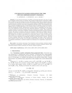
Figure 1: For evaluation reasons, given a reference motion sequence (left), the system extracts the necessary trajectories (middle) and reconstructs (right) the motion of the character based on those trajectories.
[Mousas et al. 2014b], for motion deformation [Min et al. 2009], interactive creation of a characters pose using a mouse [Grochow et al. 2004][Wei and Chai 2011] or control of human actions using vision-based tracking [Chai and Hodgins 2005], real-time human motion control with inertial sensors [Liu et al. 2011] or accelerometer sensors [Tautges et al. 2011], building physically-valid motion models for human motion synthesis [Wei et al. 2011], for quantifying natural human motion [Ren et al. 2005] and so forth.
construction process.
3
Overview
This section presents an overview of the motion reconstruction process that is used for the evaluation process. The motion reconstruction process is divided into the following steps:
In past years, a number of researchers have developed approaches that use few constraints provided by sensors to control highdimensional human motions. For example, Shotton et al. [Shotton et al. 2011] and Wei et al. [Wei et al. 2012] used a single depth camera to track and reconstruct various human motions. Their approaches acquired no markers attached to a user’s body. However, no less than 15 control points were needed to segment the human body. Semwal et al. [Semwal et al. 1998] combined the inverse kinematics algorithm and the few constraints from eight magnetic sensors to provide an analytic solution for human motion control. Chai and Hodgins [Chai and Hodgins 2005] used six to nine retroreflective markers as the control points for online human motion reconstruction. Slyper and Hodgins [Slyper and Hodgins 2008] used five inertial sensors for real-time upper-body control. Recently, Liu et al. [Liu et al. 2011] achieved full-body human motion control using the positional and orientational constraints from six inertial sensors. Tautges et al. [Tautges et al. 2011] utilized few constraints provided by four accelerometer sensors to control full-body human motion.
Prior Modelling: The prior modelling is important in human motion reconstruction because the system should be able to automatically construct the prior learning process. The prior model is used to compute the naturalness of the human pose. It is also used to constrain the reconstructed poses to remain in the space of naturallooking. In this paper, four different covariance matrix approaches for constraining prior modelling methodology were implemented.
Motion Reconstruction: The reconstruction process can be performed either in real-time by using sensors attached to the user’s body or by using off-line methods in which input trajectories reconstruct the character’s motion. The system extracts the spatiotemporal information that is stored in an off-line process using an existing sequence of motion data. Then, the system retrieves the input trajectories [c1 , ..., ct ] (which, in this case, are trajectories retrieved from a reference motion) that contain the global position and orientation of each trajectory at each time step. These trajectories specify the desired trajectories of a certain point on the animated character. The motion reconstruction process is formulated in a MAP framework that combines the prior term encoded by the different distribution models with a likelihood term, which is retrieved from the control inputs. Figure 1 provides an example of the reconstruction process based on extraction of the necessary trajectories from a reference motion. Figure 2 represents the pipeline of the motion reconstruction process.
All of these previously mentioned methodologies are responsible for animating and reconstructing the motion of virtual characters mainly by using motion capture technologies. In general, motion reconstruction can be undertaken in both on-line and off-line applications. The development of those techniques has, as its main concern, implementation on real-time performance interfaces. Hence, the evaluation process in this paper, even if the motion is generated off-line, attempts to determine the ability to reconstruct the motion of the character based on the ability to use four different covariance matrix constraints. Hence, the results of this evaluation process provide an understanding of how possible it is to design new statistical motion models that are able to reconstruct high quality motion sequences. Finally, it should be noted that we used in this evaluation process the standard markerset, which consists of six markers (see Figure 3(c)), as have been used in various previous methodologies [Chai and Hodgins 2005][Liu et al. 2011]. We assume that such a markerset can satisfy the required assumptions to understand how each of the covariance matrix constraints reacts to the motion re-
Evaluation: The evaluation process has two main steps. First, a single action of the character is reconstructed by assigning only actions that are similar to those contained in the database - such as reconstructing a walking motion sequence by using a walking motion dataset - to the prior term of the motion reconstruction process. The same procedure is then repeated although it may use the entire
100
apply the EM) for mixtures of factor analyzers is used. The determinant and the inverse of the covariance matrix are efficiently computed using two identities as follows: |A + BC| = |A| × |I +CA−1 B|
(2)
(A + BCD)−1 = A−1 − A−1 B(C−1 + DA−1 B)DA−1
(3)
Using these identities, the inverses and determinants of d × d and diagonal matrices are computed, rather than the full D×D matrices, which would results in a lower performance by the system. Thus, the equations are computed as follows:
Figure 2: The pipeline of the motion reconstruction process.
|Ψ + ΛΛT | = |Ψ| × |I + ΛT Ψ−1 Λ| (Ψ + ΛΛT )−1 = Ψ−1 − Ψ−1 Λ(I + ΛT Ψ−1 Λ)−1 ΛT Ψ−1
amount of data. Finally, each reconstructed motion is evaluated using the leave-one-out cross validation method. Both methodologies are repeated in various combinations of input data that are retrieved from the input trajectories.
4
4.1.2
This section presents both the covariance matrix constraint techniques used for the evaluation process and the MAP framework used to reconstruct human motion.
(6)
A mixture of Gaussians (MOG), in which the covariance matrices are of this type, is termed a “mixture of probabilistic principal component analyzers” [Tipping and Bishop 1999a]. Principal component analysis [Jolliffe 2005][Tipping and Bishop 1999b] (PCA) appears as a limiting case if the mixture has only one component and the variance approaches zero, i.e., σ 2 → 0 [Roweis 1998]. Let U be the D × d matrix with the eigenvectors of the data covariance matrix, where d has the largest eigenvalues, and let V be the diagonal matrix with the corresponding eigenvalues on its diagonal. Then, the maximum likelihood estimate of Λ is given by Λ = UV 1/2 . For probabilistic principal component analysis (PPCA), the number of parameters is also O(Dd), as it is for FA.
Constraining the Covariance Matrix
To highlight the difference between PCA and FA, assume the following. Using PCA, arbitrarily rotate the original basis of the space. The covariance matrix that is obtained for the variables that correspond to the new basis is still of the PCA type. Thus the class of PCA models is closed to rotation, which is not the case for FA. If some of the data dimensions are scaled, the scaled FA covariance matrix will still be of the FA type. Thus, the class of FA models is closed to non-uniform scaling of the variables, which is not the case for PCA models. If the relative scale of the variables is not considered to be meaningful, an FA model may be preferable to a PCA model, and vice versa if relative scale is important.
Factor Analysis
Factor analysis (FA) is a parametric statistical model that represents high-dimensional data using the low-dimensional data of hidden factors. In general, the covariance matrices in FA are constrained to assume the following form: Σ = Ψ + ΛΛT
Principal Component Analysis
Σ = σ 2 I + ΛΛT where σ > 0
A majority of techniques have been proposed in recent years to constrain the covariance matrix. Among the best known of those are factor analysis, principal component analysis, the k-subspaces and isotropic techniques, which are compared in this evaluation. Various other statistical models also have been proposed for human motion reconstruction. Some of them are examined in the articles by Bowden et al. [Bowden et al. 2000] for reconstructing human motion from monocular image sequences, and [Bowden 2000] for learning and reconstructing human motion based on statistical models. The approaches that were used in this evaluation are described below. In addition, in the following subsections, I denotes the identity matrix, Ψ denotes a diagonal matrix, and Λ denotes a D × d matrix, where d < D. A detailed explanation of the covariance matrix constraints can be found in [Verbeek ].
4.1.1
(5)
In the principal component analysis (PCA) [Jolliffe 2005][Tipping and Bishop 1999b], the constraints are similar to those of FA, but the matrix Ψ is further constrained to be a multiple of the identity matrix as follows:
Motion Reconstruction
4.1
(4)
4.1.3
k-Subspaces
The k-subspaces technique provides the ability to further constrain the covariance matrix so that the norm of all columns of Λ is equal to the following:
(1)
Σ = σ 2 I + ΛΛT with ΛΛT = ρ 2 I and σ , ρ > 0
The d columns of Λ are often referred to as the “factor-loading matrix”. Each column of Λ can be associated with a latent variable. In the diagonal matrix, Ψ, the variance of each data coordinate is modelled separately, and additional variance is added in the directions spanned by the columns of Λ. The covariance matrix is specified by the number of parameters equal to O(Dd). To solve the mixture of factor analyzers (MFA), the expectation-maximization (EM) algorithm (see reference [Ghahramani and Hinton 1996] for how to
(7)
This type of covariance matrix was used in [Verbeek et al. 2002] to create a non-linear dimension-reduction technique. The number of parameters is O(Dd). Using this type of covariance matrix with EM to train an MOG creates an algorithm known as k-subspaces [Kambhatla and Leen
101
1993][de Ridder 2001] under the following conditions: (i) all mixing weights are equal, i.e., πs = 1/k, and (ii) the σs and ρs are equal for all mixture components, i.e., σs = σ and ρs = ρ. Then, taking the limit as σ → 0, k-subspaces are obtained. The term k-subspaces refers to the k linear subspaces that are spanned by the columns of Λs . The k-subspaces algorithm iterates in the two following steps:
where K denotes a constant of the mixture components used, and πk is the weighted variable that is assigned to each component of the mixture model.
Step 1: Assign each data point to the subspace that best reconstructs the data vector (in terms of squared distance between the data point and the projection of the data point on the subspace).
The motion reconstruction process that is based on the previously presented covariance matrix restriction techniques can be formulated in a maximum a posteriori (MAP) framework. In this case, let ct be the input data retrieved from the input trajectories of the reference motion that must be reconstructed at the current t − th frame. By combining the current control trajectories, ct provided by input markerset of the reference motion sequence, and the constructed probabilistic model of previous m reconstructed poses Q˜ = [q˜t−1 , ..., q˜t−m ], the system reconstructs the current pose, q∗ , in a constrained MAP framework that is represented as follows:
4.2
Step 2: For every subspace, compute the PCA subspace of the assigned data to obtain the updated subspace. 4.1.4
Isotropic
Probabilistic Reconstruction
˜ q∗ = arg max p(qt |ct , Q)
The final constrain process of the covariance matrix is based on the isotropic technique. This shape of the covariance matrix is the shape that is most constrained. It is mathematically represented by the following: Σ = σ 2 I where σ > 0 (8)
qt
(11)
where p(·|·) denotes the conditional probability. Using Bayes’ rule, one obtains: ˜ ˜ q∗ = arg max p(ct |qt , Q)p(q (12) t , Q) qt
This model is termed an isotropic or spherical variance because the variance is equal in all directions. It requires a single parameter σ . In general, if all components share the same variance, σ 2 , and that variance approaches zero, the posterior of the components for a given data vector tends to put all of the mass on the component closest to the data vector by Euclidean distance [Bishop 1995]. This means that the E-step becomes to finding the closest component for all data vectors. The expectation procedure counts the term for the closest component. For the M-step, this means that the centers of the components, µs , are found by averaging all of the data vectors that are closest. This simple case of the EM algorithm coincides exactly with the k-means algorithm. Taking the Σ-diagonal, and thus letting all variables be independently distributed, is also a popular constraint, which yields O(d) parameters. 4.1.5
˜ given ct , Now, assuming that qt is conditionally independent of Q, the following is obtained: ˜ q∗ ≈ arg max p(ct |qt )p(qt , Q) qt
In this case, by applying the negative logarithm to the posterior ˜ the constrained MAP problem is distribution function, p(qt |ct , Q), converted into an energy minimization problem as follows: ˜ q∗ = arg min − ln p(ct |qt ) + − ln p(qt , Q) qt | {z } | {z } Elikelihood
The Mixture Model
4.2.1
Likelihood Distribution
The likelihood estimation process is modelled on the basis of input trajectories, ct , obtained from the input trajectories. If Gaussian noise with a standard deviation of σd is considered, the likelihood term is defined as follows: Elikelihood = − ln p(ct |qt )
The mixture models probabilistically partition the entire configuration space into multiple local regions, and then model the data distribution in each local region using a weighted variable for each region. The mixture model of the previously mentioned methodologies to constrain the covariance matrix is represented mathematically as follows:
∝
k f (qt ; s, ˜ z˜ − ct )k 2σd2
(15)
where the vector qt represents the reconstructed pose of the character at each time step, s˜ denotes the skeleton model, z˜ denotes the coordinates of each input trajectory, and ct are the observed data that are obtained from the defined trajectories. The function f is the forward kinematics function that maps the current pose, qt , to the global coordinates.
N
∑ πk N(·|µk , Σk )
E prior
(9)
where (·) is assigned with the reference input posture of the character. However, because the inputs are existing human poses that are contained in a database, it is necessary to consider the mixture model because all human poses form a non-linear manifold in the character configuration space. Thus, a global linear parametric model is often insufficient for capture of the non-linear structure of natural human motion. Therefore, a better solution is to use a mixture model.
p(·) =
(14)
where the first term (Elikelihood ) is the likelihood term that computes how well the reconstructed pose, qt , of the character fits the input trajectories, ct . The term (E prior ) describes the prior distribution of the human motion data. In this case, the prior distribution is what is evaluated during the motion reconstruction process.
Considering the covariance matrix that is assigned as Σ and the mean vector as µ, it is possible to compute the distribution of each model based on the form of: p(·) = N(·|µ, Σ)
(13)
(10)
k=1
102
4.2.2
Prior Distribution
According to Section 4.1.5, the mixture model that handles the prior knowledge of the existing data is represented as follows: ˜ k , Σk ) ∑ πk N(qt , Q|µ
Walking
Self db Whole db
13.672
Jumping 17.976
Punching 9.651 1.1 M
Golf Swing 6.324
Table 1: The motion sequences used for the evaluation process, for both self-reconstruction and general motion reconstruction.
K
˜ = p(qt , Q)
Datasets
(16)
k=1
where πk , µk and Σk denote the weighted scalar of the k − th component of the mixture model, the mean vector value and the covariance matrix, respectively, for each of the four different constrain processes of the covariance matrix. In general, the goal of the model learning process is to automatically find the model parameters πk , µk and Σk for k = 1, ..., K from the training data qn , n = 1, ..., N, where N is the number of poses in the database. For each different constrained model that uses these variables, the parameters are calculated separately using the EM algorithm. In these experiments, the number of mixture components (K) that are used are set at K = 50 and the dimension of the latent space (d) is set at d = 5. The values of (K) and (d) are determined empirically. However, cross-validation techniques can also be used to set the appropriate values of those parameters.
4.3
5.2
This section presents the evaluation procedure that was used in this study. In this case, the leave-one-out evaluation procedure was used. It computes the reconstructed error of a given motion by omitting one sequence from the motion data of the database, to be used as the testing sequence. Before beginning the evaluation process, the initial reconstruction error for each database of motions that is used must be computed by using the initial skeletal model that contains all 18 markers (see Figure 3(a)), with each constraint of the covariance matrix. The need to compute this error arises from the assumption that, when using statistical models to reconstruct human motion, the statistical error should be minimized. Because an error may be produced during the evaluation process, this error is estimated to result in more stable results. Based on this assumption, the computed error for each motion database and each constraining process of the covariance matrix is shown in Table 2.
Trajectory-Based Motion Reconstruction
During the runtime of the reconstruction process, the system should be able to handle the input trajectories that are assigned to each marker of the character’s body parts to reconstruct the required motion. In the evaluation process presented, a simple trajectory-based motion reconstruction is used, because it uses only the space-time information of the reference trajectories to evaluate the reconstruction processes. Each reference motion that is used for the reconstruction process is represented as M = {(ci ,t1 ), ..., (ci ,tn )}, where ci denotes the marker set that is used, and ti for i = 1, ..., n denotes the position of each marker at the i − th frame of the reference motion. Based on this representation, the space-time requirements of the input trajectories are satisfied for reconstruction of the character’s motion.
5
Evaluation and Results
Implementation, Evaluation, and Results
This section presents the implementation details of the methodology presented and the results of the evaluation.
5.1
Implementation Details
Figure 3: The initial (a) and reduced (b) markerset that was used for this evaluation process.
The evaluation process was implemented on an Intel i7 at 2.2 GHz with 8 GB of memory. Four types of motions were used. They were walking, jumping, punching, and a golf swing. Each motion sequence is represented by S = {P(t), Q(t), r1 (t), ..., rn (t)}, where P(t) and Q(t) represent the character’s root position and orientation at the t − th frame, respectively, and ri (t)|i = 1, ..., n represents the orientation of the character’s joints at the t − th frame. The motion data are stored in the database by executing the root position and orientation of each pose of the character. The number of poses used for each motion of the character is shown in Table 1. The sampling rate for these motions is 120 Hz. This method, although implemented in this application for off-line computations, could easily be implemented in real time. Based on these experiments, the applications run in real time with an average frame rate of 42 fps and a system latency of 0.023 seconds.
Once the initial error has been computed, the next step is to estimate the reconstructed error for each constraining process of the covariance matrix, while using a reduced number of markers (see Figure 3(b)). In this case, the percentage of the error is not computed by comparing the reference motion to the reconstructed motion, but is evaluated by comparison to the initial measurements that are outside of the initial reconstruction error. The reconstruction process was tested on different actions. The average computed reconstruction error was computed by degrees per joint angle per frame. That is, the tested motion sequences were pulled from the training dataset, and simulated the motion by using the defined trajectories that contain both the position and the orientation of each marker at each time step. For each einitial , which denotes the initial
103
Datasets
Walking
Self db Whole db
0.022% 0.028% 0.03% 0.036% 0.038% 0.032% Principal Component Analysis
0.033% 0.039%
the k-subspaces and the isotropic, it is possible to reconstruct motion sequences that have a grater error than with factor analysis or principal component analysis. Hence, the general advantage of the FA and PCA is based on the ability to reconstruct motions with less error while dealing with different datasets.
Self db Whole db
0.02% 0.035%
0.019% 0.026% 0.034% 0.029% k-subspaces
0.03% 0.034%
6
Self db Whole db
0.024% 0.037%
0.022% 0.029% 0.039% 0.044% Isotropic
0.035% 0.041%
Self db Whole db
0.028% 0.043%
0.032% 0.046%
0.037% 0.048%
Jumping Punching Factor Analysis
0.036% 0.052%
Golf Swing
The ability to reconstruct a virtual character’s motion based on a few input signals that are retrieved from a motion capture system has been thoroughly studied in recent years. Various solutions have been proposed to reconstruct human motion with different motion reconstruction techniques. However, in this study, an evaluation process for human motion reconstruction is presented that is based on the ability to constrain the covariance matrix of the probabilistic model that retrieves the prior learning process.
Table 2: The initial error computed for each motion database that was used for the reconstruction process, combined with the different methods that constrain the covariance matrix.
The following conclusions were derived from the experiments. First, a less-constrained covariance matrix of a probabilistic character’s motion reconstruction process is able to reconstruct highquality motions of the character, while using either a large or a small amount of data to form the prior knowledge of the system. The same results are obtained while using a small number of input trajectories, or when reconstructing a particular action of the character. Hence, the less that a covariance matrix is constrained, the less error is produced.
error based on Table 2, the reconstructed error is evaluated separately for each motion as follows: e f inal = 1 −
e × 100 einitial
(17)
where e denotes the reconstruction error that is computed while using the reduced number of markers. Thus, the results obtained from this evaluation process are illustrated in Table 3. Datasets
Walking
Jumping Punching Factor Analysis
Self db Whole db
0.99% 0.98% 0.82% 1.15% 1.12% 0.99% Principal Component Analysis
0.86% 1.05%
Self db Whole db
1.02% 1.16%
1.01% 0.84% 1.17% 1.01% k-subspaces
0.92% 1.07%
Self db Whole db
1.07% 1.22%
1.04% 1.09% 1.24% 1.29% Isotropic
1.16% 1.32%
Self db Whole db
1.11% 1.24%
1.13% 1.23%
1.19% 1.44%
1.14% 1.32%
Conclusions and Future Work
This research was a first attempt to understand how covariance matrix constraints may influence the motion reconstruction process. Even if other methodologies to reconstruct human poses have been proposed that are not included in the scope of this study, a roadmap has been provided to show where future research of human motion reconstruction should be undertaken. The authors’ future plans include generating statistical motion models to reconstruct highquality motion sequences by reducing the error while designing a high-quality motion reconstruction model that can be efficiently employed at every motion-capture interface.
Golf Swing
References A BE , Y., L IU , C. K., AND P OPOVI C´ , Z. 2006. Momentum-based parameterization of dynamic character motion. Graphical Models 68, 2, 194–211. A RIKAN , O., AND F ORSYTH , D. A. 2002. Interactive motion generation from examples. ACM Transactions on Graphics 21, 3 (July), 483–490.
Table 3: This table shows the error that was computed during the reconstruction process for the four different covariance matrix constraints that were implemented.
BADLER , N. I., H OLLICK , M., AND G RANIERI , J. 1993. Realtime control of a virtual human using minimal sensors. Presence: Teleoperators and Virtual Environments 2, 1, 82–86.
The results presented in Table 3 show that, when using motion models such as the factor analysis or the principal component analysis, higher quality motion sequences can be reconstructed because the measurement error is minimal in comparison to those of other constrained approaches of the covariance matrix. This is especially true when using the self-database of motion sequences. The second important result is based upon the ability to reconstruct the character’s motion using a smaller number of markers. In this case, it is shown that a less constrained covariance matrix can reconstruct more valid character motion for particular actions of the character, including walking, jumping, punching and golf swings. Therefore, while constraining the covariance matrix using techniques, such as
B ISHOP, C. M. 1995. Neural Networks for Pattern Recognition. Oxford University Press. B OWDEN , R., M ITCHELL , T. A., AND S ARHADI , M. 2000. Nonlinear statistical models for the 3d reconstruction of human pose and motion from monocular image sequences. Image and Vision Computing 18, 9, 729–737. B OWDEN , R. 2000. Learning statistical models of human motion. In IEEE Workshop on Human Modeling, Analysis and Synthesis, IEEE, vol. 2000.
104
B RAND , M., AND H ERTZMANN , A. 2000. Style machines. In ACM SIGGRAPH Annual Conference on Computer Graphics and Interactive Techniques, ACM, 183–192.
for the environment. In Computer Graphics International, IEEE, 156–159. M IN , J., C HEN , Y. L., AND C HAI , J. 2009. Interactive generation of human animation with deformable motion models. ACM Transactions on Graphics 29, 1, Article No. 9.
B RAND , M. 1999. Voice puppetry. In ACM SIGGRAPH Annual Conference on Computer Graphics and Interactive Techniques, ACM, 21–28.
M OUSAS , C., N EWBURY, P., AND A NAGNOSTOPOULOS , C.-N. 2014. Data-driven motion reconstruction using local regression models. In 10th International Conference on Artificial Intelligence Applications and Innovations.
B REGLER , C., C OVELL , M., AND S LANEY, M. 1997. Video rewrite: Driving visual speech with audio. In ACM SIGGRAPH Annual Conference on Computer Graphics and Interactive Techniques, ACM, 353–360.
M OUSAS , C., N EWBURY, P., AND A NAGNOSTOPOULOS , C.-N. 2014. Efficient hand-over motion reconstruction. In 22nd International Conference on Computer Graphics, Visualization and Computer Vision.
C HAI , J., AND H ODGINS , J. K. 2005. Performance animation from low-dimensional control signals. ACM Transactions on Graphics 24, 3, 686–696. R IDDER , D. 2001. Adaptive Methods of Image Processing. PhD thesis, Delft University of Technology.
¨ ¨ M ULLER , M., R ODER , T., AND C LAUSEN , M. 2005. Efficient content-based retrieval of motion capture data. ACM Transactions on Graphics 24, 3 (July), 677–685.
DE
G HAHRAMANI , Z., AND H INTON , G. E. 1996. The EM algorithm for mixtures of factor analyzers. Tech. Rep. CRG-TR-96-1, University of Toronto.
R EN , L., PATRICK , A., E FROS , A. A., H ODGINS , J. K., AND R EHG , J. M. 2005. A data-driven approach to quantifying natural human motion. ACM Transactions on Graphics 24, 3 (July), 1090–1097.
G LEICHER , M. 1998. Retargetting motion to new characters. In ACM SIGGRAPH Annual Conference on Computer Graphics and Interactive Techniques, ACM, 33–42.
ROWEIS , S. 1998. EM algorithms for PCA and SPCA. In Advances in Neural Information Processing Systems, 626–632.
G ROCHOW, K., M ARTIN , S. L., H ERTZMANN , A., AND P OPOVI C´ , Z. 2004. Style-based inverse kinematics. ACM Transactions on Graphics 23, 3 (August), 522–531.
S AFONOVA , A., AND H ODGINS , J. K. 2007. Construction and optimal search of interpolated motion graphs. ACM Transactions on Graphics 26, 3 (August), Article No. 106.
J OLLIFFE , I. 2005. Principal Component Analysis. John Wiley & Sons Ltd.
S EMWAL , S. K., H IGHTOWER , R., AND S TANSFIELD , S. 1998. Mapping algorithms for real-time control of an avatar using eight sensor. Presence: Teleoperators and Virtual Environments 7, 1, 1–21.
K AMBHATLA , N., AND L EEN , T. K. 1993. Fast nonlinear dimension reduction. In IEEE International Conference on Neural Networks, IEEE, 1213–1218.
S HIN , H. J., L EE , J., S HIN , S. Y., AND G LEICHER , M. 2001. Computer puppetry: An importance-based approach. ACM Transactions on Graphics 20, 2, 67–94.
´ C ONAIRE , C., AND O’C ONNOR , N. E. 2010. HuK ELLY, P., O man motion reconstruction using wearable accelerometers. In ACM SIGGRAPH/Eurographics Symposium on Computer Animation.
S HOTTON , J., F ITZGIBBON , A., C OOK , M., S HARP, T., F INOC CHIO , M., M OORE , R., K IPMAN , A., AND B LAKE , A. 2011. Real-time human pose recognition in parts from a single depth image. In IEEE Conference on Computer Vision and Pattern Recognition, IEEE, 1297—1304.
K EOGH , E., PALPANAS , T., Z ORDAN , V. B., G UNOPULOS , D., AND C ARDLE , M. 2004. Indexing large human-motion databases. In Very Large Databases, VLDB Endowment, vol. 30, 780–791.
S LYPER , R., AND H ODGINS , J. K. 2008. Action capture with accelerometers. In ACM SIGGRAPH/Eurographics Symposium on Computer Animation, Eurographics Association, 193–199.
KOVAR , L., AND G LEICHER , M. 2003. Flexible automatic motion blending with registration curves. In ACM SIGGRAPH/Eurographics Symposium on Computer Animation, Eurographics Association, 214–224.
¨ TAUTGES , J., Z INKE , A., K R UGER , B., BAUMANN , J., W E ¨ BER , A., H ELTEN , T., M ULLER , M., S EIDEL , H.-P., AND E BERHARDT, B. 2011. Motion reconstruction using sparse accelerometer data. ACM Transactions on Graphics 30, 3, Article No. 18.
KOVAR , L., G LEICHER , M., AND P IGHIN , F. 2002. Motion graphs. ACM Transactions on Graphics 21, 3, 473–482. L EE , J., AND S HIN , S. Y. 1999. A hierarchical approach to interactive motion editing for human-like figures. In ACM SIGGRAPH Annual Conference on Computer Graphics and Interactive Techniques, ACM, 39–48.
T IPPING , M. E., AND B ISHOP, C. M. 1999. Mixtures of probabilistic principal component analyzers. Neural computation 11, 2, 443–482.
L I , Y., WANG , T., AND S HUM , H. Y. 2002. Motion texture: A two-level statistical model for character motion synthesis. ACM Transactions on Graphics 21, 3 (July), 465–472.
T IPPING , M. E., AND B ISHOP, C. M. 1999. Probabilistic principal component analysis. Journal of the Royal Statistical Society, Series B..
L IU , H., W EI , X., C HAI , J., H A , I., AND R HEE , T. 2011. Realtime human motion control with a small number of inertial sensors. In Symposium on Interactive 3D Graphics and Games, ACM, 133–140.
BASTEN , B., AND E GGES , A. 2012. Motion transplantation techniques: A survey. IEEE Computer Graphics and Applications 32, 3, 16–23.
VAN
M E´ NARDAIS , S., M ULTON , F., K ULPA , R., AND A RNALDI , B. 2004. Motion blending for real-time animation while accounting
V ERBEEK , J. Mixture Models for Clustering and Dimension Reduction. PhD thesis, Universiteit van Amsterdam.
105
¨ , B. 2002. CoordiV ERBEEK , J. J., V LASSIS , N., AND K R OSE nating principal component analyzers. In Artificial Neural Networks, Springer Berlin Heidelberg, 914–919. W EI , X. K., AND C HAI , J. 2011. Intuitive interactive humancharacter posing with millions of example poses. IEEE Computer Graphics and Applications 31, 4, 78–88. W EI , X., M IN , J., AND C HAI , J. 2011. Physically valid statistical models for human motion generation. ACM Transactions on Graphics 30, 3, Article No. 19. W EI , X., Z HANG , P., AND C HAI , J. 2012. Accurate realtime fullbody motion capture using a single depth camera. ACM Transactions on Graphics 31, 6, Article No. 188. W ITKIN , A., AND P OPOVI C´ , Z. 1995. Motion warping. In ACM SIGGRAPH Annual Conference on Computer Graphics and Interactive Techniques, ACM, 105–108. Y IN , K., AND PAI , D. K. 2003. Footsee: An interactive animation system. In ACM SIGGRAPH/Eurographics Symposium on Computer Animation, Eurographics Association, 329–338.
106