Exact Inference for Gaussian Process Regression in ...

Exact Inference for Gaussian Process Regression in case of Big Data with the Cartesian Product Structure Belyaev Mikhail MIKHAIL . BELYAEV @ DATADVANCE . NET Institute for Information Transmission Problems, Bolshoy Karetny per. 19, Moscow, 127994, Russia

arXiv:1403.6573v1 [stat.ME] 26 Mar 2014

DATADVANCE, llc, Pokrovsky blvd. 3, Moscow, 109028, Russia PreMoLab, MIPT, Institutsky per. 9, Dolgoprudny, 141700, Russia Burnaev Evgeny EVGENY. BURNAEV @ DATADVANCE . NET Institute for Information Transmission Problems, Bolshoy Karetny per. 19, Moscow, 127994, Russia DATADVANCE, llc, Pokrovsky blvd. 3, Moscow, 109028, Russia PreMoLab, MIPT, Institutsky per. 9, Dolgoprudny, 141700, Russia Kapushev Yermek ERMEK . KAPUSHEV @ DATADVANCE . NET Institute for Information Transmission Problems, Bolshoy Karetny per. 19, Moscow, 127994, Russia DATADVANCE, llc, Pokrovsky blvd. 3, Moscow, 109028, Russia

Abstract Approximation algorithms are widely used in many engineering problems. To obtain a data set for approximation a factorial design of experiments is often used. In such case the size of the data set can be very large. Therefore, one of the most popular algorithms for approximation — Gaussian Process regression — can be hardly applied due to its computational complexity. In this paper a new approach for Gaussian Process regression in case of factorial design of experiments is proposed. It allows to efficiently compute exact inference and handle large multidimensional data sets. The proposed algorithm provides fast and accurate approximation and also handles anisotropic data.

1. Introduction Gaussian Processes (GP) have become a popular tool for regression which has lots of applications in engineering problems (Rasmussen & Williams, 2006). They combine flexibility of being able to approximate a wide range of smooth functions with simple structure of Bayesian inference and interpretable hyperparameters. GP regression algorithm has O(N 3 ) time complexity and O(N 2 ) memory complexity, where N is a size of the training sample. For large training sets (ten thousands or more)

construction of GP regression becomes intractable problem on current hardware. There is significant amount of research concerning sparse approximation of GP regression reducing run-time complexity to O(M 2 N ) for some M N (for example, M can be the size of a subsample used for sparse approximation). There are also methods based on Mixture of GPs and Bayesian Machine Committee. Overview of these methods can be found in (Rasmussen & Williams, 2006; Rasmussen & Ghahramani, 2001; Quiñonero-Candela & Rasmussen, 2005). Reduced run-time and memory complexity can be achieved not only by means of sparse approximations and Mixtures of GPs but also by taking into account a structure of a design of experiments. In engineering problems they often use a factorial design (Montgomery, 2006). That is there are several groups of variables, in each group variables take values from some discrete finite set. Such sets and corresponding groups of variables are called factors. Number of different values in a factor is called factor size and the values themselves are called levels. The Cartesian product of factors forms the training set. When the factorial design of experiments is used the size of the data set can be very large (as it grows exponentially with dimension of input variables). There are several methods based on splines which consider

Exact Inference for Gaussian Process Regression in case of Big Data with the Cartesian Product Structure

this special structure of the given data (Stone et al., 1997). A disadvantage of these methods is that they work only with one-dimensional factors and can’t be applied to a more general case when factors are multidimensional. Another shortcoming is that such approaches don’t have approximation accuracy evaluation procedure.

There is another problem which we are likely to encounter. Factor sizes can vary significantly. Engineers usually use large factors sizes if corresponding input variables have big impact on function values otherwise the factors sizes are likely to be small, i.e. the factor sizes are often selected using knowledge from a subject domain (Rendall & Allen, 2008). For example, if it is known that dependency on some variable is quadratic then the size of this factor will be 3 as a larger size is redundant. Difference between factor sizes can lead to degeneracy of the GP model. We will refer to this property of data set as anisotropy. In this paper we describe an approach that takes into account factorial nature of the design of experiments in general case of multidimensional factors and allows to efficiently calculate exact inference of GP regression. We also discuss how to choose initial values of parameters for the GP model and regularization in order to take into account possible anisotropy of the training data set. 1.1. Approximation problem

2 εi ∼ N (0, σnoise ).

0.7 0.6 0.5 0.4 0.3 0.2

1

0.1 0 0.9

0.5 0.8

0.7

0.6

0.5

0.4

0.3

0.2

0.1

0

(1)

1.2. Factorial design of experiments In this paper a special case is considered when the design of experiments is factorial. Let us refer to sets of points sk = {xkik ∈ Xk }nikk=1 , Xk ⊂ Rdk , k = 1, K as factors. A set of points S is referred to as a factorial design of experi-

0

x2

x1

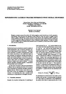
Figure 1. Example of a multidimensional factor. In the figure x1 is a usual one-dimensional factor and (x2 , x3 ) is a 2-dimensional factor.

ments if it is a Cartesian product of factors S = s1 × s2 × · · · × sk = K {[x1i1 , . . . , xK iK ], {ik = 1, . . . , nk }k=1 }.

(2)

PK The elements of S are vectors of a dimension d = i=1 di and theQsample size is a product of sizes of all factors K N = i=1 ni . If all the factors are one-dimensional S is a full factorial design. But in a more general case factors are multidimensional (see example in Figure 1). Note that in this paper we do not consider categorical variables, factorial design is implemented across continuous real-valued features. 1.3. Gaussian Process Regression GP regression is a Bayesian approach where a prior distribution over continuous functions is assumed to be a Gaussian Process, i.e. f | X ∼ N (µ, Kf ),

Let f (x) be some unknown smooth function. The task is given a data set D = {(xi , yi ), xi ∈ Rd , yi ∈ R}N i=1 of N pairs of inputs xi and outputs yi construct an approximation fˆ(x) of the function f (x) where outputs yi are assumed to be noisy with additive i.i.d. Gaussian noise: yi = f (xi ) + εi ,

0.8

x3

There are also several approaches for GP regression on a lattice based on block Toeplitz covariance matrix with Toeplitz blocks and circulant embedding (Zimmerman, 1989; Chan & Wood, 1997; Dietrich & Newsam, 1997). Such methods have O(N log N ) time complexity and O(N ) memory complexity. They can be used only if all the factors are one-dimensional and after monotonic transformation of each factor (levels of each factor should be equally spaced). However, in the case of multidimensional factors the covariance matrix doesn’t have the desired structure (it should be block Toeplitz with Toeplitz blocks) and therefore these approaches can’t be generalized for such design of experiments.

1 0.9

(3)

where f = (f (x1 ), f (x2 ), . . . , f (xN )) is a vector of outputs, X = (xT1 , xT2 , . . . , xTN )T is a matrix of inputs, µ = (µ(x1 ), µ(x2 ), . . . , µ(xN )) is a mean vector for some function µ(x), Kf = {k(xi , xj )}N i,j=1 is a covariance matrix for some a priori selected covariance function k. Without loss of generality we make the standard assumption of zero-mean data. Also assume that we are given observations with Gaussian noise yi = f (xi ) + εi ,

2 εi ∼ N (0, σnoise )

For a prediction of f (x∗ ) at new unseen data point x∗ the posterior mean conditioned on the observations y =


(y1 , y2 , . . . , yN ) at training inputs X is used fˆ(x∗ ) = k(x∗ )T K−1 y y,

(4)

where k(x∗ ) = (k(x∗ , x1 ), . . . , k(x∗ , xN ))T , Ky = 2 I and I is an identity matrix. For approxiKf + σnoise mation accuracy evaluation the posterior variance is used cov(fˆ(x∗ )) = k(x∗ , x∗ ) − k(x∗ )T K−1 y k(x∗ ).

(5)

Usually for GP regression a squared exponential covariance function is used ! d X 2 2 (i) (i) 2 k(xp , xq ) = σf exp − (6) θi (xp − xq ) . i=1

Let us denote the vector of hyperparameters θi by θ = (θ1 , . . . , θd ). To choose the hyperparameters of our model we consider the log likelihood 1 1 log p(y | X, θ, σf , σnoise ) = − yT K−1 log |Ky |− y y− 2 2 N log 2π − 2 (7) and optimize it over the hyperparameters (Rasmussen & Williams, 2006). The runtime complexity of learning GP regression is O(N 3 ) as we need to calculate inverse of Ky , its determinant and derivatives of the log likelihood.

2. Proposed approach 2.1. Tensor and related operations For further discussions we will use tensor notation, so let’s introduce definition of a tensor and some related operations. A tensor Y is a K-dimensional matrix of size n1 × n2 × · · · × nK (Kolda & Bader, 2009): Y = {yi1 ,i2 ,...,iK , {ik =

1, . . . , nk }K k=1 }.

(8)

By Y (j) we will denote a matrix consisting of elements of the tensor Y whose rows are 1 × nj slices of Y with fixed indices ij+1 , . . . , iK , i1 , . . . , ij−1 and altering index ij = 1, . . . , nj . In case of 2-dimensional tensor it holds that Y (1) = Y T and Y (2) = Y. Now let’s introduce multiplication of a tensor by a matrix along the direction i. Let B be some matrix of size ni × n0i . Then the product of the tensor Y and the matrix B along the direction i is a tensor Z of size n1 × · · · × ni−1 × n0i × ni+1 × · · · × nK such that Z (i) = Y (i) B. We will denote

this operation by Z = Y ⊗i B. For a 2-dimensional tensor Y multiplication along the first direction is a left multiplication by matrix Y ⊗1 B = B T Y, and along the second direction — is a right multiplication Y ⊗2 B = YB. Multiplication of a tensor by a matrix along some direction is closely related to the Kronecker product. Let’s consider an operation vec which for every multidimensional matrix Y returns a vector containing all elements of Y. An inner product of tensors Y and Z is the inner product of vectors vec(Y) and vec(Z) hY, Zi = hvec(Y), vec(Z)i . For every multidimensional matrix Y of size n1 × n2 × · · · × nK and ni × pi size matrices Bi , i = 1, . . . , K the following identity holds (Kolda & Bader, 2009) (B1 ⊗ B2 · · · ⊗ BK )vec(Y) = T vec(Y ⊗1 B1T · · · ⊗K BK ),

(9)

where symbol ⊗ denotes the Kronecker product. Let’s compare a complexity of the right and the left hand sides of (9). For simplicity we assume that Qall the matrices Bi are quadratic of size ni × ni and N = ni . Then computation of the left hand side of (9) requires N 2 operations (of additions and multiplications) not taking into account complexity of the PKronecker product while the right hand side requires N i ni operations. 2.2. Computing inference In this section an efficient way to compute inverse of a covariance matrix will be described as well as calculation of the log likelihood, its derivatives, the predictive mean and the covariance matrix using introduced tensor operations. Covariance function (6) can be represented as a product of covariance functions each depending only on variables from one factor k(xp , xq ) =

K Y

ki (xip , xiq ),

(10)

i=1

where xip , xiq ∈ Rdi belong to the same factor si . For the squared exponential function we have ki (xip , xiq ) = Pdi (j) 2 (j),i (j),i 2 (j),i 2 σf,i exp − j θi xp − xq , where xp is a j-th component of xip . Note that in general case covariance functions ki are not necessarily squared exponential, they can be of different types for different factors. It allows to take into account special features of factors (knowledge from a subject domain) if they are known. In such case the function defined by (10) is still a valid covariance function being the product of separate covariance functions. From

Exact Inference for Gaussian Process Regression in case of Big Data with the Cartesian Product Structure (1)

(d )

write K−1 y y as

now on we will denote by θi = (θi , . . . , θi i ) the set of hyperparameters for covariance function of the i-th factor and let θ = (θ1 , . . . , θK ).

K−1 y y =

Such form of the covariance function and the factorial design of experiments allows us to represent the covariance matrix as the Kronecker product

K O i=1

= vec Kf =

K O

Ki ,

Ui

! "K O

# 2 Di + σnoise I

!−1 ×

i=1

×vec(Y ⊗1 U1 · · · ⊗K UK ) = (Y ⊗1 U1 · · · ⊗K UK ) ∗ D−1 ⊗1 ⊗1 UT1 · · · ⊗K UTK , (13)

(11) where D is a tensor by transforming the diago N constructed 2 nal of matrix k Dk + σnoise I into a tensor.

i=1

where Ki is a covariance matrix defined by the ki covariance function computed at points from the i-th factor si .

The elements of the tensor D are eigenvalues of the matrix Ky , therefore its determinant can be calculated as

The Kronecker product of matrices can be efficiently inverted due to the following property

|Ky | =

Y

Di1 ,...,iK .

(14)

i1 ,...,iK

(A ⊗ B)−1 = A−1 ⊗ B −1

Proposition 1. The computational complexity of the log likelihood (7), where K−1 y y and |Ky | are calculated using (13) and (14), is ! K K X X 3 O ni + N ni . (15)

if A and B are invertible matrices. If A has size na × na and B has size nb × nb then the left side of the above equation requires O(n3a n3b ) operations while the right hand side requires only O(n3a + n3b ) operations and this is much less. 2 However, we have to invert the matrix Ky = Kf +σnoise I. For this we will use the Singular Value Decomposition (SVD)

i=1

Proof. Let’s calculate the complexity of computing K−1 y y using (13).PComputation of the matrices Ui and Di requires O( i n3i ) operations. Multiplication P of the tensor Y by the matrices Ui requires O(N i ni ) operations. Further, component-wise product of the obtained tensor and the tensor D−1 requires O(N ) operations. And complexity of multiplication of the result P by the matrices Ui is again O(N i ni ). The determinant, calculated by equation (14), requires O(N ) operations. PKThus, the overall PK complexity of computing (13) is O( i=1 n3i + N i=1 ni ).

Ki = Ui Di UTi , where Ui is an orthogonal matrix of eigenvectors of matrix Ki and Di is a diagonal matrix of eigenvalues. Using the properties of the Kronecker product and representing an identity matrix as Idi = Ui UTi we obtain

K−1 y

=

K O i=1

Ui

! "K O

!−1

# Di +

2 σnoise I

i=1

K O

! UTi

i=1

(12) Computing SVD for all Ki requires O( k n3k ) operations. Calculation of the Kronecker product in (12) has complexity O(N 2 ). So, this gives us overall complexity O(N 2 ) for calculation of expressions for the log likelihood, the predictive mean and the covariance. It is faster than the straightforward calculations, however it can be improved. P

Equations (4), (5), (7) for GP regression do not require explicit inversion of Ky . In each equation it is multiplied by vector y (or k∗ ). So, we will compute K−1 y y instead of explicitly inverting Ky and then multiplying it by the vector y. Let Y be a tensor containing values of the vector y such that vec(Y) = y. Now using identities (9) and (12) we can

i=1

.

For more illustrative estimate of the computational complexity suppose that ni N (number of factors is large and their In this case it holds that P sizes are close). 1 O(N i ni ) = O(N 1+ K ) and this is much less than O(N 3 ). To optimize the log likelihood over the hyperparameters we use a gradient based method. The derivatives of the log likelihood with respect to the hyperparameters take the form ∂ (log p(y|X, σf , σnoise )) = ∂θ 1 1 T −1 0 −1 0 − Tr(K−1 y K ) + y Ky K Ky y, 2 2

(16)

where θ is one of the hyperparameters of covariance function (component of θi , σnoise or σf,i , i = 1, . . . , d) and


K0 =

∂K . K0 is also the Kronecker product ∂θ

K0 = K1 ⊗ · · · ⊗ Ki−1 ⊗

Table 1. Runtime (in seconds) of tensored GP and original GP algorithms.

∂Ki ⊗ Ki+1 ⊗ · · · ⊗ KK , ∂θ

ORIGINAL

where θ is a parameter of the i-th covariance function. Denoting by A a tensor such that vec(A) = K−1 y y the second term in equation (16) can be efficiently computed using the same technique as in (13): 1 T −1 0 −1 y Ky K Ky y = 2 A, A ⊗1 KT1 ⊗2 · · · ⊗i−1 KTi−1 ⊗i

64 160 432 1000 2000 10240 64000 160000 400000

(17)

∂KTi ⊗i+1 KTi+1 ⊗i+2 · · · ⊗K KTK ∂θ

GP

0.8 2.69 14.31 120.38 970.21 — — — —

TENSORED

GP

0.16 0.16 0.74 1.02 1.11 33.18 74.9 175.15 480.14

.

The complexity of calculating this term of derivative is the same as the complexity of equation (13). Now let’s compute the first term ! K O −1 0 Tr(Ky K ) = Tr Ui D−1 i=1

2.3. Anisotropy K O

! UTi

! K0

=

i=1 K O

= Tr D−1

!! UTi K0i Ui

=

i=1

* −1

=

diag D

, diag

K O

!+ Ui K0i Ui

=

i=1

* =

−1

diag D

+ K O 0 , diag (Ui Ki Ui ) , i=1

(18)

where diag of diagonal elements of a matrix N A is a vector 2 A, D = i Di + σnoise I. The computational complexity of this derivative term is the same as the computational complexity of equation (17). Thus, we obtain Proposition 2. The computational complexity calculating derivatives K of the log likelihood K P 3 P O ni + N ni . i=1

of is

In this section we will consider an anisotropy problem. As it was mentioned in an engineering practice factorial designs are often anisotropic, i.e. sizes of factors differ significantly. It is a common case for the GP regression to become degenerate in such situation. Suppose that the given design of experiments consists of two one-dimensional factors with sizes n1 and n2 . Assume that n1 n2 . Then one could expect the length-scale for the first factor to be much greater than the length-scale for the second factor (or θ1 θ2 ). However, in practice we often observe the opposite θ1 θ2 . This happens because the optimization algorithm stacks in a local maximum during maximization over the hyperparameters as the objective function (the log likelihood) is non-convex with lots of local maxima. We get an undesired effect of degeneracy: in the region without training points the approximation is constant and it has sharp peaks at training points. This situation is illustrated in Figure 3 (compare with the true function in Figure 4). (i) −1 (i) Let us denote length-scales as lk = θk . To incorporate our prior knowledge about factor sizes into regression model we introduce prior distribution on the hyperparameters θ:

i=1

Table 1 contains training times for original GP and proposed GP regression for different sample sizes. The experiments were conducted on a PC with Intel i7 2.8 GHz processor and 4 GB RAM. For original GP we used GPML Matlab code (Rasmussen & Nickisch, 2010). We also adopted GPML code to use tensor operations. The results illustrate that the proposed approach is much more faster than the original GP and allows to make approximations using extremely large data sets.

(i)

(i)

(i)

(i)

θk − ak bk − ak

∼ Be(α, β), {i = 1, . . . , dk }K k=1 ,

(19)

(i)

i.e. prior on hyperparameter θk is a beta distribution h iwith (i)

(i)

parameters α and β scaled to some interval ak , bk

.

Exact Inference for Gaussian Process Regression in case of Big Data with the Cartesian Product Structure 1

The log likelihood then has the form

0

1 1 log p(y | X, θ, σf ,σnoise ) = − yT K−1 log |Ky |− y y− 2 2 ! (i) (i) X θk − ak N − log 2π+ (α − 1) log + (i) (i) 2 bk − ak k,i !! (i) (i) θk − ak +(β − 1) log 1 − (i) − d log(B(α, β)), (i) bk − ak (20)

where B(α, β) is a beta function.

(i)

−2 −3 −4 −5 −6

a=b=2 0

0.5

1 x

(i)

long to some interval ak , bk (or length-scales lk to h i (i) −1 (i) −1 , ak belong to the interval bk ). This choice of prior allows to prohibit too small and too large lengthscales excluding possibility to degenerate (if intervals of allowed length-scales are chosen properly).

1.5

2

Figure 2. Logarithm of Beta distribution probability density function, rescaled to [0.01, 2] interval, with parameters α = β = 2.

2.5

Numerous references use gamma distribution as a prior, e.g. (Neal, 1997). Preliminary experiments showed that GP regression models with gamma prior often degenerates. So, in this work we use prior with compact support. By (i) introducing such prior hwe restrict i parameters θk to be(i)

log(PDF)

−1

GP regression training set

2 1.5 1 0.5 0 −0.5 −1 1 0.5 1

0

0.5 0

−0.5 x2

−1

−0.5 −1

x1

It seems reasonable that for an approximation to fit the training points the length-scale is not needed to be much less than the distance between points. That’s why we (i) choose the lower bound for the length-scale lk to be ck ∗ min ||x(i) − y (i) || and the upper bound for

Figure 3. Degeneracy of the GP model in case of anisotropic data set. The length-scales for this model are l1 = 0.286, l2 = 0.033 whereas factor sizes are n1 = 15, n2 = 4.

the length-scale to be Ck ∗ max ||x(i) − y (i) ||. The value

It is also important to choose reasonable initial values of hyperparameters in order to converge to a good solution during parameters optimization. The kernel-widths for different factors should have different scales because corresponding factor sizes have different number of levels. So it seems reasonable to use average distance between points in a factor as an initial value −1 1 (i) (i) (i) θk = max(x ) − min (x ) . (21) x∈sk nk x∈sk

x,y∈sk ,x(i) 6=y (i)

x,y∈sk

ck should be close to 1. If it is chosen too small we are taking risks to overfit the data by allowing small lengthscales. If ck is too large we are going to underfit the data by allowing only large length-scales and forbidding small ones. Constants Ck must be much greater than ck to permit large length-scales and preserve flexibility. In this work we used ck = 0.5 and Ck = 100. Such values of ck and Ck worked rather good in our test cases. Parameters of beta distribution was set to α = β = 2 to get symmetrical probability distribution function (see Figure 2). We don’t know a priori large or small should be the values of GP parameters, so prior distribution should impose nearly the same penalties for the intermediate values of the parameters. As it can be seen from Figure 2 the chosen distribution does exactly what is needed. Figure 5 illustrates approximation of the GP regression with introduced prior distribution (and initialization described in Section 2.4). The hyperparameters were chosen such that the approximation is non-degenerate.

2.4. Initialization

3. Experimental results Proposed algorithm was tested on a set of test functions (Evoluationary computation pages — the function testbed; System optimization — testroblems). The functions have different input dimensions from 2 to 6 and the sample sizes N varied from 100 to about 200000. For each function several factorial anisotropic training sets were generated. We will test the following algorithms: GP with tensor computations (tensorGP), GP with tensor computations and prior


2.5

distribution (tensorGP-reg), the sparse pseudo-point input GP (FITC) (Snelson & Ghahramani, 2005). For FITC method we used GPML Matlab code (Rasmussen & Nickisch, 2010). Number of inducing points of FITC algorithm varied from M = 500 for small samples (up to 5000 points) to M = 70 for large samples (about 105 points) in order to obtain approximation in reasonable time (complexity of FITC algorithm is O(M 2 N )). For tensorGP and tensorGPreg we adopted GPML code to use tensor operations, proposed prior distribution and initialization.

True function training set

2 1.5 1

To assess quality of approximation a mean squared error was used

0.5 0 −0.5 −1 1

MSE = 0.5 1

0

0.5 0

−0.5 −1

x2

−0.5 −1

1

N test X

Ntest

i=1

(fˆ(xi ) − f (xi ))2 ,

(22)

where Ntest = 50000 is a size of test set. The test sets were generated randomly.

x1

A large set of problems (number of problems is about 40) was used to test the algorithms. Usual “test problem vs. MSE” plot will be confusing for large set of problems as it will look like noisy graph. To see a picture of the overall performance of algorithms on such test problems set we use Dolan-Moré curves (Dolan & Moré, 2002). The idea of Dolan-Moré curves is as follows. Let tp,a be an error of an a-th algorithm on a p-th problem and rp,a be a performance ratio tp,a rp,a = . min(tp,s )

Figure 4. True function.

s

Then Dolan-Moré curve is a graph of ρa (τ ) function where ρa (τ ) = 2.5

which can be thought of as a probability for the a-th algorithm to have performance ratio within factor τ ∈ R+ . The higher the curve ρa (τ ) is located the better works the corresponding algorithm. ρa (1) is a number of problems on which the a-th algorithm showed the best performance.

tensorGP−reg training set

2 1.5 1 0.5 0 −0.5 −1 1 0.5

1

0

0.5 0

−0.5 x2

−1

1 size{p : rp,a ≤ τ }, np

As expected tensorGP performs better than FITC as it uses all the information containing in the training sample. Introduced prior distribution is more suited for anisotropic data that’s why GP with such prior (tensorGP-reg) performs even better (see Figure 6).

−0.5 −1

x1

Figure 5. The GP regression with proposed prior distribution and initialization.

To compare run-time performances of the algorithms we plotted Dolan-Mor’e curves where instead of approximation error the training time was used (see Figure 7). Here we see that tensorGP and tensorGP-reg outperform FITC algorithm. 3.1. Rotating disc problem In this section we will consider a real world problem of rotating disc shape design. Such kind of problems often


0.9 0.8 0.7

ρa (τ)

0.6 0.5 0.4

Figure 8. Rotating disc parametrization.

0.3 0.2 FITC tensorGP tensorGP−reg

0.1 0

0

0.2

0.4

0.6

0.8

1

1.2

1.4

1.6

1.8

2

log(τ)

Figure 6. Approximations accuracies comparison. Dolan-Moré curves for tensorGP, tensorGP-reg and FITC algorithms in logarithmic scale. The higher lies the curve the better performs the corresponding algorithm. Figure 9. Rotating disc objectives.

arises during aircraft engine design and in turbomachinery (Armand, 1995). In this problem a disc of an impeller is considered. It is rotated around the shaft. The geometrical shape of the disc considered here is parameterized by 6 variables x = (h1 , h2 , h3 , h4 , r2 , r3 ) (r1 and r4 are fixed), see Figures 8 and 9. The task of an engineer is to find such geometrical shape of the disc that minimizes disc’s weight and contact pressure p1 between the disc and the shaft while constraining the maximum radial stress Srmax to be less than some threshold. The physical model of a rotating disc is described in (Armand, 1995) and it was adopted to the disc shape presented in Figures 8, 9 in order to calculate the contact pressure p1 and the maximum radial stress Srmax .

1 0.9 0.8 0.7

ρa (τ)

0.6 0.5 0.4 0.3 0.2

FITC tensorGP tensorGP−reg

0.1 0

0

0.2

0.4

0.6

0.8

1

1.2

1.4

1.6

1.8

log(τ)

Figure 7. Run-times comparison. Dolan-Moré curves for tensorGP, tensorGP-reg and FITC algorithms in logarithmic scale. The higher lies the curve the better performs the corresponding algorithm.

2

It is a common practice to build approximations of objective functions in order to analyze them and perform optimization (Forrester et al., 2008). So, we applied developed in this work tensorGP-reg algorithm and FITC to this problem. The design of experiments was full factorial, number of points in each dimension was [1, 8, 8, 3, 15, 5], i.e x1 was fixed. Number of points in factors differ significantly and the generated data set is anisotropic. The overall number of points in the training sample was 14 400. Figures 10 and 11 depict 2D slices of contact pressure approximations along x5 , x6 variables. As you can see FITC model degenerates while tensorGP-reg provides smooth


100

100

50

50 p1

150

p1

150

0

0

−50

−50 FITC training set test set

−100 350 300

tensorGP−reg training set test set

−100 350 300

250

250 200 150 100 50 x5

650

600

550

500

450

400

350

200 150 100 50

x6

Figure 10. 2D slice along x5 and x6 variables (other variables are fixed) of FITC approximation with 500 inducing inputs. It can be seen that the approximation degenerates.

and accurate approximation.

4. Conclusion Gaussian Processes are often used for building approximations for small data sets. However, knowledge about the structure of the given data set can contain important information which allows us to efficiently compute exact inference even for large data sets. Introduced prior distribution combined with reasonable initialization has proven to be an efficient way to struggle degeneracy in case of anisotropic data.

x5

650

600

550

500

450

400

350

x6

Figure 11. 2D slice along x5 and x6 variables (other variables are fixed) of tensorGP-reg approximation. It can be seen that tensorGP-reg provides accurate approximation.

lation of stationary gaussian processes through circulant embedding of the covariance matrix. SIAM J. Sci. Comput., 18(4):1088–1107, July 1997. ISSN 1064-8275. Dolan, Elizabeth D. and Moré, Jorge J. Benchmarking optimization software with performance profiles. Mathematical Programming, 91(2):201–213, January 2002. Evoluationary computation pages — the function testbed. Laappeenranta University of Technology. URL http://www.it.lut.fi/ip/evo/ functions/functions.html.

Algorithm proposed in this paper takes into account the special factorial structure of the data set and is able to handle large multidimensional samples preserving power and flexibility of GP regression. Our approach has been successfully applied to toy and real problems including the rotating disc shape design.

Forrester, Alexander I. J., Sobester, Andras, and Keane, Andy J. Engineering Design via Surrogate Modelling - A Practical Guide. J. Wiley, 2008.

References

Montgomery, Douglas C. Design and Analysis of Experiments. John Wiley & Sons, 2006. ISBN 0470088109.

Armand, S. C. Structural Optimization Methodology for Rotating Disks of Aircraft Engines. NASA technical memorandum. National Aeronautics and Space Administration, Office of Management, Scientific and Technical Information Program, 1995. Chan, Grace and Wood, Andrew T.A. Algorithm as 312: An algorithm for simulating stationary gaussian random fields. Journal of the Royal Statistical Society: Series C (Applied Statistics), 46(1):171–181, 1997. ISSN 14679876. Dietrich, C. R. and Newsam, G. N. Fast and exact simu-

Kolda, Tamara G. and Bader, Brett W. Tensor decompositions and applications. SIAM Review, 51(3):455–500, 2009.

Neal, Radford M. Monte carlo implementation of gaussian process models for bayesian regression and classification. arXiv preprint physics/9701026, 1997. Quiñonero-Candela, Joaquin and Rasmussen, Carl Edward. A unifying view of sparse approximate gaussian process regression. The Journal of Machine Learning Research, 6:1939–1959, 2005. Rasmussen, Carl E. and Williams, Christopher. Gaussian Processes for Machine Learning. MIT Press, 2006.


Rasmussen, Carl Edward and Ghahramani, Zoubin. Infinite mixtures of gaussian process experts. In In Advances in Neural Information Processing Systems 14, pp. 881– 888. MIT Press, 2001. Rasmussen, Carl Edward and Nickisch, Hannes. Gaussian processes for machine learning (gpml) toolbox. J. Mach. Learn. Res., 11:3011–3015, December 2010. ISSN 1532-4435. Rendall, T.C.S. and Allen, C.B. Multi-dimensional aircraft surface pressure interpolation using radial basis functions. Proc. IMechE Part G: Aerospace Engineering, 222:483 – 495, 2008. Publisher: IMechE. Snelson, Edward and Ghahramani, Zoubin. Sparse gaussian processes using pseudo-inputs. In Advances in Neural Information Processing Systems 18, pp. 1257–1264. MIT press, 2005. Stone, Charles J., Hansen, Mark, Kooperberg, Charles, and Truong, Young K. Polynomial splines and their tensor products in extended linear modeling. Ann. Statist, 25: 1371–1470, 1997. System optimization — testroblems. Swiss International Institute of Technology. URL http: //www.tik.ee.ethz.ch/sop/download/ supplementary/testproblems/. Zimmerman, DaleL. Computationally efficient restricted maximum likelihood estimation of generalized covariance functions. Mathematical Geology, 21(7):655–672, 1989. ISSN 0882-8121.