Experiments in Speaker Verification using Factor

Experiments in Speaker Verification using Factor Analysis Likelihood Ratios Patrick Kenny and Pierre Dumouchel Centre de recherche informatique de Montr´eal (CRIM) {pkenny, pdumouch}@crim.ca

Abstract We report the results of some speaker verification experiments on the NIST 1999 and NIST 2000 test sets using factor analysis likelihood ratio statistics. For the experiments on the 1999 test set we had to use a mismatched training set, namely Phases 1 and 2 of the Switchboard II corpus, to train the factor analysis model. Our results on this test set are are comparable to (but not better than) the best results that have been attained with standard methods (GMM likelihood ratios and handset detection). In order to experiment with well matched training and test sets, we used half of the target speakers in the NIST 2000 evaluation for testing and a disjoint set of speakers taken from Switchboard II, Phases 1 and 2 for training. In this situation we obtained an equal error rate of 7.2% and a minimum detection cost of 0.028. These figures represent an improvement of about 25% over standard methods.

1. Introduction Simply stated, the basic problem in speaker verification is to decide whether two utterances have been uttered by the same speaker or by different speakers. Put another way, one has to decide whether the differences between the two utterances are better accounted for by inter-speaker variability or by what might be termed inter-session variability, that is, the variability exhibited by a given speaker from one recording session to another. This type of variability may be attributable either to channel effects or to intra-speaker variation (the speaker’s health or emotional state for example) but channel effects are presumably more important in general. In state of the art methods of speaker verification interspeaker variability is assumed to be of primary importance (classical MAP estimation of GMM’s [1, 2] is implicitly based on a model of inter-speaker variability, namely a Gaussian prior on speaker-dependent GMM supervectors) but it has long been recognized that inter-session variability is a serious problem [3, 4]. In face recognition it has been found that models of intra-person variability (which capture differences in posture and illumination in different images of the same subject) are capable of high performance even when inter-person variability is not modeled at all [5]. This suggests that a systematic model of inter-session variability could prove to be useful in speaker verification, particularly if it is integrated with an effective model of inter-speaker variability. In [6] we proposed eigenchannel MAP as a model of inter-session variability and in [7] we showed how it could be integrated with standard models of inter-speaker variability, namely classical MAP and eigenvoice MAP [8], to produce a joint model of inter-speaker and inter-session variability which we referred to as a factor analysis of speaker and channel effects. The present article reports the results of recent experiments in text-independent speaker verification using factor analysis likelihood ratio statistics.

Our original motivation in developing the factor analysis model was to use model adaptation techniques developed for speech recognition to perform channel adaptation of speaker models in speaker recognition. Two difficulties arise here. Firstly, very little data may be available for channel adaptation. For example, test utterance durations range from 15 to 45 seconds in the NIST restricted data evaluations. Secondly, model adaptation techniques developed for speech recognition conflate inter-speaker and channel variability so that, although they are usually thought of as performing speaker adaptation, they may be performing channel adaptation in some situations and speaker adaptation in others. In order to be effective for speaker recognition, model adaptation techniques must be capable of adapting speaker models to the channel effects in a test utterance without adapting them to the speaker in the test utterance. This raises a very challenging estimation problem. For example, several authors have suggested compensating for channel effects in speaker recognition by applying affine transformations. These transformations can be applied either in the feature space [9, 10, 11] or in the model space space [12] with equivalent results so this method can be regarded as a type of model adaptation. The question is how to estimate the parameters of such an affine transformation given a hypothesized speaker and test utterance. One procedure which has been suggested [10] is to estimate the affine transformation in such a way as to match the global first and second order statistics of the speaker’s enrollment data with those of test utterance but it is unclear whether this performs channel adaptation or speaker adaptation. Another possibility is to use MLLR which is a maximum likelihood estimation procedure for affine transformations applied in the model space. This is widely used in speech recognition but it does not seem to work for channel adaptation of speaker models in speaker recognition [13]. On the other hand, it should be possible in principle to constrain affine transformations to perform channel adaptation rather than speaker adaptation by means of a suitable prior distribution on the transformation parameters so that MAPLR [14] might work. However since these parameters would have to be estimated from short test utterances the lack of adaptation data would still be a problem. Eigenvoice and EMAP approaches represent a different type of model adaptation method that has been developed in speech recognition specifically in order to deal with situations where very small amounts of adaptation data are available (as in on-line speaker adaptation). EMAP is a Bayesian speaker adaptation technique which, like classical MAP, is based on a Gaussian prior distribution on speaker-dependent HMM or GMM supervectors. It differs from classical MAP in that the supervector covariance matrix — let us call it B — is assumed to be full rather than diagonal so that it takes account of the correlations between different Gaussians in a speaker model. Thus whereas classical MAP only adapts the Gaussians which are observed

in the adaption data, EMAP adapts all of the Gaussians even in situations where only a small fraction of them are observed. Eigenvoice methods are based on the assumption that the supervector covariance matrix B is of low rank so that speaker supervectors are constrained to lie in a linear manifold of low dimension which is known as the speaker space. This type of constraint facilitates very rapid speaker adaptation since only a small number of free parameters need to be estimated, namely the coordinates of a speaker’s supervector relative to a basis of the speaker space. (The eigenvectors of B which correspond to non-zero eigenvalues — the ‘eigenvoices’ — constitute such a basis.) We will refer to these free parameters as speaker factors. Combining the eigenvoice assumption with EMAP gives eigenvoice MAP [8]. This type of model adaptation can be modified to tackle the problem of channel-adaptation of speaker models for speaker recognition by assuming that the speakerand channel-dependent supervectors for different recordings of a given speaker have a Gaussian distribution centered on the speaker’s supervector. If the covariance matrix of this distribution is tied across speakers and C denotes the common value, then C can be estimated by the same methods as the supervector covariance matrix in eigenvoice MAP but whereas the covariance matrix B models inter-speaker variation, C models inter-session variation. This is the basic idea in eigenchannel MAP [6]. The eigenvalues of C (like the eigenvalues of B) generally decay exponentially so C can be taken to be of low rank in practice. This makes it possible to perform channel adaptation of speaker models on very short test utterances. It is natural to think of the range of C as the channel space and to define channel factors analogously to speaker factors. The development of eigenchannel MAP in [6] was incomplete because it addressed the first of these questions but not the second: 1. How is it possible to adapt a speaker model to the channel effects in a test utterance without performing speaker adaptation? 2. How is it possible to estimate a speaker model in a way which is immune to the channel effects in the speaker’s enrollment data? In order to provide an answer to the second question it seems to be necessary to integrate eigenchannel MAP with a model of inter-speaker variability. The simplest possibility is to use the prior in eigenvoice MAP for this purpose. This amounts to assuming that each speaker- and channel-dependent supervector can be decomposed into a sum of two supervectors, one of which lies in the speaker space and the other in the channel space. Given an enrollment recording for a speaker we can disentangle the speaker and channel effects in the corresponding speaker- and channel-dependent supervector by calculating the joint posterior distribution of the speaker and channel factors. Suppressing the contribution of the channel factors to the supervector gives (in theory at least) an estimate of the speaker’s supervector which is immune to the channel effects in the enrollment recording. The factor analysis model in [7] takes this idea one step further by incorporating the prior for classical MAP as well as the prior for eigenvoice MAP in order to compensate for the rank deficiency problem in eigenvoice MAP [8]. The factor analysis model and the models in [15, 16] are formally quite similar. In [16], the basic assumption is that each speaker- and channel-dependent supervector is a sum of a speaker-dependent supervector and a channel-dependent supervector. The major difference is that the factor analysis model

treats the channel space as a continuum whereas in [16] channel effects are quantized so that there is a discrete set of channel supervectors (one for electret handsets, another for carbon and so forth). For this approach the second question above presents no particular difficulty since it can be tackled by applying the appropriate type of channel compensation in enrollment as well as in testing [16]. Although our original goal in developing the factor analysis model was to tackle the problem of adapting speaker GMM’s to the channel effects in a test utterance with a view to carrying out speaker verification experiments using conventional GMM likelihood ratio statistics, we discovered other likelihood ratio statistics along the way which are more natural in that they are constructed using the likelihood function of the factor anaylsis model itself rather than the GMM likelihood function. In [7] we reported the results of some preliminary experiments with one of these likelihood ratio statistics. We used the Switchboard Cellular Part I corpus for training the factor analysis model and the NIST 2001 cellular one speaker detection task for testing. We discovered after the fact that the target speakers for this task are all contained in Switchboard Cellular Part I so the results of these experiments cannot be taken at face value. Our purpose in the present paper is to report the results of some recent experiments with the factor analysis model which are not tainted by this defect.

2. Factor Analysis The factor analysis model combines the priors underlying classical MAP, eigenvoice MAP and eigenchannel MAP so we begin by reviewing these and showing how a single prior can be constructed which embraces all of them. We assume a fixed GMM structure containing a total of C mixture components. Let F be the dimension of the acoustic feature vectors. 2.1. Speaker and channel factors To begin with let us ingore the question of inter-session variability and assume that each speaker s can be modeled by a single supervector M (s) which is independent of channel effects. We can combine the priors for classical MAP and eigenvoice MAP by assuming that there is a rectangulare matrix v of low rank and a diagonal matrix d such that, for a randomly chosen speaker s, M (s) = m + vy(s) + dz(s) (1) where m is the speaker-independent supervector and y(s) and z(s) are assumed to be independent and to have standard normal distributions. In other words, M (s) is assumed to be normally distributed with mean m and covariance matrix vv ∗ +d2 . This is a factor analysis model in the sense of [17]. The components of y(s) are ‘speaker factors’ and v is a ‘factor loading matrix’. The ‘speaker space’ is the affine space defined by translating the range of vv ∗ by m. If d = 0 then all speaker supervectors are contained in the speaker space; in the general case (d 6= 0), the term dz(s) serves as a residual which compensates for the fact that this type of subspace constraint may not be realistic. In order to incorporate channel effects, suppose we are given recordings h = 1, . . . , H(s) of a speaker s. For each recording h, let M h (s) denote the corresponding speaker- and channel-dependent supervector. We assume that the difference between M h (s) and M (s) can be accounted for by a vector of channel factors xh (s) having a standard normal distribution. That is, we assume that there is a rectangular matrix u of low

rank (the loading matrix for the channel factors) such that  M (s) = m + vy(s) + dz(s) M h (s) = M (s) + uxh (s)

(2)

for each recording h = 1, . . . , H(s). So if RC is the number of channel factors and RS the number of speaker factors, the factor analysis model is specified by a quintuple Λ of the form (m, u, v, d, Σ) where m is CF ×1, u is CF ×RC , v is CF ×RS and d and Σ are CF ×CF diagonal matrices. To explain the role of Σ, fix a mixture component c and let Σc be the corresponding block of Σ. For each speaker s and recording h, let Mhc (s) denote the subvector of M h (s) corresponding to the given mixture component. We assume that, for each speaker s and recording h, observations drawn from mixture component c are distributed with mean Mhc (s) and covariance matrix Σc . In the case d = 0 and u = 0 the factor analysis model reduces to the prior for eigenvoice MAP. In the case where u = 0 and v = 0 we obtain the prior for classical MAP. (The ‘relevance factors’ in [2] are the diagonal entries of d−2 Σ. Thus, although its role is rarely spelt out explicitly, the diagonal matrix d is the key to the success of state of the art methods of speaker verification.) If we assume that M (s) has a point distribution instead of the Gaussian distribution specified by (1) and that this point distribution is different for different speakers, we obtain the prior for eigenchannel MAP. Classical MAP speaker adaptation has the property that it behaves like speaker-dependent training as the amount of adaptation data for a speaker increases. The residual term dz(s) is included in the factor analysis model in order to ensure that it inherits the asymptotic behavior of classical MAP but it is costly in terms of both mathematical and computational complexity. The reason for this is that, although the increase in the number of free parameters is relatively modest since (unlike u and v) d is assumed to be diagonal, introducing z(s) greatly increases the number of hidden variables. On the other hand if d = 0, the model is quite simple since the basic assumption is that each speaker- and channel-dependent supervector is a sum of two supervectors one of which is contained in the speaker space and the other in the channel space.1 We will use the term Principal Components Analysis (PCA) to refer to the case d = 0. 2.2. The likelihood function Suppose that we are given a set of hyperparameter estimates Λ and a set of recordings for a speaker s indexed by h = 1, . . . , H(s). For each recording h, assume that each frame has been aligned with a mixture component and let Xh (s) denote the collection of labeled frames for the recording. Let X (s) be the vector obtained by concatenating the observable variables X1 (s), . . . , XH(s) (s) and let X(s) be the vector obtained by concatenating the unobservable variables x1 (s), . . . , xH(s) (s), y(s), z(s). If X(s) were given we could write down M h (s) and calculate the (Gaussian) likelihood of Xh (s) for each recording h so the calculation of the likelihood of X (s) would be straightforward. Let us denote this conditional likelihood by PΛ (X (s)|X(s)). Since the values of the hidden variables are not given, calculating the likelihood of 1 It is not necessary to assume that the speaker space and the channel spaces are orthogonal in order to ensure uniqueness of this decomposition. Uniqueness follows from the fact that the range of uu∗ and the range of vv ∗ , being low dimensional subspaces of a very high dimensional space, (typically) only intersect at the origin.

X (s) requires evaluating the integral Z PΛ (X (s)|X)N (X|0, I)dX

(3)

where N (X|0, I) is the standard Gaussian kernel N (x1 |0, I) · · · N (xH(s) |0, I)N (y|0, I)N (z|0, I). We denote the value of this integral by PΛ (X (s)). In the classical MAP case a similar type of likelihood function was proposed for constructing likelihood ratio statistics in speaker verification in [18] (but note that the authors’ use of the word factor is different from ours). 2.3. Speaker-independent hyperparameter estimation If we are given a training set in which each speaker is recorded in multiple sessions the hyperparameters Λ can be estimated by EM algorithms which guarantee that the total likelihood of the training data increases from one iteration to the next. (The Q total likelihood of the training data is s PΛ (X (s)) where s ranges over the speakers in the training set.) We refer to these as speaker-independent hyperparameter estimation algorithms (or simply as training algorithms) since they consist in fitting (2) to the entire collection of speakers in the training data rather than to an individual speaker. One estimation algorithm, which we will refer to simply as maximum likelihood estimation, can be derived by extending Proposition 3 in [8] to handle the hyperparameters u and d in addition to v and Σ. Our experience with it has been that it tends to converge very slowly. Another algorithm can be derived by using the divergence minimization approach to hyperparameter estimation introduced in [19]. This seems to converge much more rapidly but it has the property that it keeps the orientation of the speaker and channel spaces fixed so that it can only be used if these are well initialized. (A similar situation arises when the divergence minimization approach is used to estimate inter-speaker correlations. See the remark following Proposition 3 in [19].) We have experimented with the maximum likelihood approach on its own and with the maximum likelihood approach followed by divergence minimization. With one notable exception, we obtained essentially the same performance in both cases (even though the hyperparameter estimates are quite different). 2.4. Adapting from one speaker population to another In order to use the speaker-independent hyperparameter estimation algorithms, we need a training set in which there are multiple recordings of each speaker. The enrollment data provided by NIST for the one speaker detection evaluations are not adequate for this purpose since there is just one (or at best two) enrollment recordings for each target speaker. So in order to test our model on, say, the NIST 1999 data we need an ancilliary training set such as the union of Switchboard II, Phases 1 and 2. Thus in practice there may be a mismatch between the training speaker population and the target speaker population. We have attempted to deal with this problem by first estimating a full set of hyperparameters m, u, v, d and Σ on the ancilliary training set and then, holding u and Σ fixed, re-estimating m, v and d on the enrollment data for the target speakers. In other words, we keep the hyperparameters associated with channel space fixed and re-estimate only the hyperparameters associated with the speaker space. It turns out to be important to use the divergence minimization rather than the maximum likelihood

approach in this situation. That is, it is necessary to keep the orientation of the speaker space fixed as well as that of the channel space rather than change it to fit the target speaker population (in order to avoid overtraining on the very limited amount of enrollment data provided by NIST). 2.5. Enrolling a speaker In order to construct the likelihood ratio statistic that we will use for speaker verification, we also need a speaker-dependent hyperparameter estimation algorithm. For this we assume that, for a given speaker s and recording h,  M (s) = m(s) + v(s)y(s) + d(s)z(s) (4) M h (s) = M (s) + uxh (s). That is, we make the hyperparameters m, v and d speakerdependent but we continue to treat u and Σ as speakerindendent. Given enrollment data for the speaker s, we estimate the speaker-dependent hyperparameters m(s), v(s) and d(s) by first using the speaker-independent hyperparameters and the enrollment data to calculate the posterior distribution of M (s) and then adjusting the speaker-dependent hyperparameters to fit this posterior. (More specifically, we find the prior of the form m(s) + v(s)y(s) + d(s)z(s) which is closest to the posterior in the sense that the divergence is minimized. This is just the minimum divergence estimation algorithm applied to a single speaker in the case where u and Σ are held fixed.) Thus m(s) is an estimate of the speaker’s supervector when channel effects are abstracted and d(s) and v(s) measure the uncertainty in this estimate. Set Λ(s) = (m(s), u, v(s), d(s), Σ). 2.6. The likelihood ratio statistic Given speaker-independent hyperparameters Λ and enrollment data for a speaker s, we can estimate a set of speaker-dependent hyperparameters Λ(s) as we have just explained. Given speech data X uttered by a test speaker t, to test the hypothesis that t = s against the hypothesis that t 6= s we use the likelihood ratio PΛ(s) (X ) 1 log (5) T PΛ (X ) where T is the duration of the test utterance. Evaluating this likelihood ratio statistic could be prohibitively expensive in the context of the NIST evaluations because it is desirable to have a large number of speaker factors in order to discriminate between speakers. The computation needed to evaluate the numerator in (5) essentially boils down to calculating the Cholesky decomposition of a matrix of dimension (RS + RC ) × (RS + RC ) constructed from v(s) and u. (Recall that RC is the rank of u and RS is the rank of v and of v(s).) Reducing the rank of v(s) to manageable proportions by discarding the minor eigenvalues of v(s)v ∗ (s) alleviates the computational burden of this Cholesky decomposition. Since v(s) captures the uncertainty in the values of the speaker factors after enrollment, most of the eigenvalues of v(s)v ∗ (s) are small so this is a reasonable approximation. The same problem arises in evaluating the denominator of (5) but this can be avoided altogether by using t-norm score normalization.

3. Training and Test Sets In order to experiment properly with the factor analysis model we need a test set and a training set which is disjoint from the test set but reasonably well matched with respect to both

speaker and channel characteristics. Unfortunately it is very difficult to satisfy this requirement using the NIST evaluation sets because of the way they have been extracted from the Switchboard corpora [20]. For example, using the NIST 2002 or 2003 evaluation data for testing and Switchboard Cellular Part I for training would not be appropriate since the evaluation data consists principally of CDMA transmissions and there would be essentially no CDMA transmissions in the training data. Among recent test sets, the best choice seems to be to use the test set for 1999 (which is extracted from the Switchboard II, Phase 3 corpus) along with Switchboard II, Phases 1 and 2 for training. The Switchboard II corpora consist of land line data with roughly equal proportions of ‘same number’ and ‘different number’ calls so there should be no mismatch where channel characteristics are concerned. However there is a mismatch between the training and target speaker populations because the training speakers are from the American Midwest and Northeast and the target speakers from the South. We found that, under these conditions, factor analysis likelihood ratios are capable of achieving results on the 1999 test set which are as good as (but no better than) the best results that have been attained with standard GMM likelihood ratios and handset detection using unwarped cepstral coefficients as acoustic features. Our efforts to improve on these results by adapting the factor analysis model to the target speaker population using the strategy outlined in Section 2.4 were largely unrewarded but we did find that much better performance could be achieved by using Switchboard II, Phase 3 as the training set (that is, by cheating in the same way as in our preliminary experiments [7]). This suggests that good results could be attained if a well matched training set were available but since we were unable to test this hypothesis on the 1999 test set we used a subset of the NIST 2000 test set instead. The 2000 test set is unusually large since it involves a thousand target speakers. These speakers were drawn from both Phase 1 and Phase 2 of Switchboard II and the test utterances were all extracted from different number calls. We constructed the test set for our final experiments by discarding every second target speaker in the 2000 test set and we constructed a training set using speakers in Switchboard II, Phases 1 and 2 which were not included in our test set. We found that the factor analysis model performed very well in this situation. Traditionally NIST defines a ‘primary condition’ for the annual evaluations. In 1999 and 2000 the primary conditions were defined in such a way that only the electret portions of the test sets were used in the evaluations. We did not impose the primary condition restrictions in our experiments since we were interested to see how the factor analysis model would perform on a mixture of electret and carbon data.

4. Implementation Issues Using large numbers of speaker and/or channel factors creates problems in speaker-independent estimation of the hyperparameters. The principal computational bottleneck here is in calculating the posterior distribution of the hidden variables (that is, PΛ (X(s)|X (s))) for each training speaker s. If the number of recordings of the speaker is large (the ideal situation) and there are large numbers of speaker and channel factors then this calculation may not be practically feasible unless d = 0. In our preliminary experiments on the NIST 2001 cellular test set using the Switchboard Cellular Part I corpus for training [7] we did not encounter any difficulties here because we used only 40 speaker and 40 channel factors but for most of our experiments

on the NIST 1999 and NIST 2000 test data we did have to impose the restriction d = 0. (Even with this restriction training can still be very time consuming. For example we found that training a PCA model with 300 speaker factors and 100 channel factors on a Switchboard database takes almost one half real time per EM iteration on a 2 GHz PC.) Calculating the posterior distribution of the hidden variables is only problematic in training the factor analysis model on large training sets; there is no difficulty in introducing d in adapting the speaker-independent hyperparameters from the training speaker population to a NIST target speaker population (since the enrollment data for each target speaker consists of just one or two recordings). We found that in order to avoid excessive I/O overheads in evaluating on a NIST data set, the best scenario is to load the speaker-dependent hyperparameters for a given target speaker s into memory and then perform all of the verification trials in which the speaker s is hypothesized. This produces results sorted by target speaker but it is a simple matter to resort them by test utterance. Evaluating the likelihood ratio statistics for a given test utterance and a given set of hypothesized target speakers requires a Viterbi or Baum-Welch alignment of the test data. We used Baum-Welch alignments and speaker-independent or genderdependent GMM’s for this purpose. An obvious advantage of using only gender-dependent GMM’s for alignment is that a given test utterance need only be aligned once (rather than once for each hypothesized speaker as required by the usual GMM approach). Thus the number of Gaussians in the GMM is not really a major issue for us. As for signal processing, speech data was sampled at 8 kHz and 12 liftered mel frequency cepstral coefficients and an energy parameter were calculated at a frame rate of 10 ms. The acoustic feature vector consisted of these 13 parameters together with their first derivatives. Cepstral mean subtraction was not performed since the channel factors in the factor analysis model can account for convolutional noise. Similarly, the energy feature was not normalized. We did not use feature warping in this study because, notwithstanding its effectiveness with traditional GMM likelihood ratios, this technique may suppress information which is useful for the factor analysis model. Since silences were excised from the NIST 1999 and NIST 2000 enrollment and test data, we used a silence detector to prepare the training data for our experiments. Unlike most other authors, we did not use handset detection for our experiments (except to break down some of our results).

5. Experiments In this section we will first report results obtained on the NIST 1999 test set (which was extracted from Switchboard II, Phase 3) by training PCA models on Switchboard II, Phases 1 and 2. As we mentioned in Section 3, the training and test sets for these experiments are mismatched. In order to see how well a PCA model is capable of performing if the training and test sets are well matched, we also carried out some experiments on a subset of the NIST 2000 test set (which was extracted from both Phases 1 and 2 of Switchboard II) where we used a subset of the NIST 2000 target speaker population for testing and a disjoint set of speakers from Switchboard II, Phases 1 and 2 for training.

5.1. Databases For each target speaker in the 1999 evaluation, the enrollment data consisted of about one minute of speech from each of two different conversations conducted over the same phone line. There were 309 female target speakers and 230 males. There were 3,420 test utterances and 11 trials per utterance for a total of 37,620 verification trials. For most of our experiments on the 1999 test set we used only the female data which consisted of 1,972 test utterances. We used one of the two enrollment recordings for each of the target speakers (5 hours of data in the female case, 4 in the male) to train two gender-dependent GMM’s each having 2,048 Gaussians. We used the Switchboard II, Phases 1 and 2 corpora to construct two training sets (one male and one female) for training PCA models. We excluded all speakers who were included in the 1999 evaluation.2 This left 625 female training speakers and 528 male. For computational reasons we did not use all of the conversation sides for these speakers but we took care to balance A and B sides. There were 128 hours of female training data (after excising silences) and 94 hours of male data. For the NIST 2000 evaluation two minutes of enrollment data extracted from a single conversation side were provided for each target speaker (457 males and 546 females). There were 6,052 test utterances extracted from different number conversation sides and 11 trials per utterance for a total of 66,572 verification trials. In order to design the training and test sets for our final experiments we began by excluding from the test set every second target speaker as well as all target speakers whose NIST identification numbers were not in the set of Switchboard II, Phases 1 and 2 identification numbers. This gave us a set of 453 target speakers (203 male and 250 female). We selected a disjoint set consisting of 341 male and 385 female speakers from Switchboard II, Phases 1 and 2 for training. For each training speaker we used up to 20 conversation sides, giving 121 hours of training data in the female case and 96 hours in the male. Finally we constructed our test set from the NIST 2000 test set by excluding trials which involved speakers other than our 453 target speakers or test utterances which had been extracted from one of the conversation sides that we used in training. This left us with 27,438 verification trials (13,516 male and 13,922 female) involving 5,207 test utterances. Of these, 24% were recorded with carbon button handsets (compared with 23% of 6,052 test utterances in the test set as a whole). Thus the results we will report on our test set can be compared with results obtained by other authors on the NIST 2000 test set as a whole (that is, without the primary condition restriction). 5.2. A toy experiment The most promising strategy for dealing with the mismatch between the training and target speaker populations in experimenting on the 1999 test set seems to be to use a large number of speaker factors in the hope of generating a speaker space which is large enough to accommodate the target speakers as well as the training speakers. However if we use a large number of speaker factors then computational considerations force us to take d = 0 (as we mentioned in Section 4) and to make an 2 Care is needed in making this determination because, although NIST uses the Switchboard speaker identification numbers, some speakers have aliases. This situation arises when two sets of enrollment data, one carbon and one electret, are supplied for a speaker.

approximation in evaluating the likelihood ratio statistic (5) (as we mentioned in Section 2.6). In order to see if our model was capable in principle of performing well under these conditions we performed an experiment on the female test data where we trained a PCA model on the female portion of Switchboard II, Phase 3. (This violates the evaluation protocol in the same way as our preliminary experiments [7] since the 1999 test data was extracted from Switchboard II, Phase 3.) In estimating the hyperparameters we limited ourselves to 10 conversation sides per training speaker (this gave us 63 hours of female training data after excising silences) and we estimated a PCA model with 300 speaker factors and 50 channel factors using the maximum likelihood training algorithm. In testing we used t-norm score normalization with 50 t-norm speakers per test utterance. In order to evaluate the likelihood ratio statistic (5) we reduced the rank of v(s) from 300 to 50 for each target speaker s. Under these conditions we obtained a DCF of 0.016 and an EER of 4.8% on the female portion of the test set.3 This indicates that a PCA model together with the approximation used in evaluating the likelihood ratio statistic can indeed perform well at least if the training and test sets are perfectly matched. Although these results seem to be very good, it turns out that, as in the case of conventional GMM systems (and human listeners for that matter [21]), the performance on different number trials is much poorer than on same number trials. This is apparent from Table 1 where we have broken down the results in the same way as in [2, 22].

SNST DNST DNDT

DCF 0.006 0.016 0.033

5.3. Results on the 1999 test set We used 500 speaker factors and 50 channel factors for our experiments on the 1999 test set. As in the toy experiment, we reduced the rank of v(s) to 50 for each target speaker s in evaluating the likelihood ratio statistic (5) and we used 50 t-norm speakers for each test utterance. We first performed a series of experiments on the female portion of the test set using the female training set extracted from Switchboard II, Phases 1 and 2 to estimate PCA models. Our aim was to investigate the effectiveness of the two types of estimation algorithm (maximum likelihood and minimum divergence) in training the PCA models and in adapting them to the target speaker population. The results are summarized in Lines 1–5 of Table 2. Line 1 gives the results obtained with maximum likelihood training detection cost function (DCF) is given by min (0.99PF A + 0.1PM )

1 2 3 4 5 6 7

Training ML PCA ML PCA ML PCA MD PCA MD PCA MD PCA MD PCA

Adaptation — ML PCA MD PCA — MD PCA MD PCA + d MD FA

DCF 0.037 0.055 0.037 0.036 0.036 0.031 0.030

EER 9.9% 15.2% 10.8% 10.4% 10.6% 9.2% 9.2%

Table 2: Results on the female portion of the 1999 test set obtained by training on Switchboard II, Phases 1 and 2 for various training and adaptation regimes. ML = maximum likelihood estimation, MD = minimum divergence estimation, PCA = principal components analysis, FA = factor analysis. For the experiment reported in Line 6 we took the adapted PCA model from Line 5 and turned it into a factor analysis model simply by setting 1 Σ (7) 16 as [2] would suggest. (As we mentioned, in the classical MAP case the relevance factors in [2] are the diagonal entries of d−2 Σ.) This turned out to be a good choice; estimating a factor analysis model from the enrollment data using this model as an initialization and the minimum divergence adaptation algorithm gave essentially the same results (Line 7). Comparing the results in Lines 6 and 7 with those in Line 5 shows that factor analysis can outperform principal components analysis. The approach taken in Line 7 has the advantage that relevance factors do not have to be pulled out of a hat but comparing Line 6 with Line 7, Line 4 with Line 5 and Line 1 with Line 3 shows that our attempts to palliate the mismatch problem by adapting to the target speaker population using the approach indicated in Section 2.4 were unsuccessful. Furthermore the results in Line 2 shows that this approach can actually be harmful if maximum likelihood estimation is used in place of minimum divergence estimation (as we mentioned in Section 2.4). We replicated the experiment in Line 7 on the male portion of the 1999 test set, obtaining a DCF of 0.029 and an EER of 10.2%. Pooling male and female trials gave worse results than keeping them separate, namely a DCF of 0.033 and an EER of 10.9% so it appears that using common thresholds for male and female trials is suboptimal for the factor analysis model. It is quite likely that this is due to the disparity in the sizes of the male and female training sets. (There are generally more females than males in the Switchboard corpora.) For comparison, results on the 1999 test set without the primary condition restriction are reported in [22] and in [2] where an EER of 10% was obtained. d2 =

EER 2.2% 4.8% 10.0%

Table 1: Breakdown of results on the female portion of the 1999 test set obtained by training on Switchboard II, Phase 3. SNST indicates same number, same type (electret or carbon), DNST indicates different number, same type and DNDT indicates different number, different type.

3 The

of the PCA model without any adaptation to the target speaker population. These results are reasonably good but not nearly as good as in our toy experiment which suggests that the mismatch between the training and target speaker populations may be a problem. The performance (as measured by the DCF) with minimum divergence training (Line 4) and with minimum divergence adaptation (Lines 3 and 5) was essentially the same as in Line 1.

(6)

where PM and PF A denote the miss probability and the false alarm probability at a given operating point and the minimum is taken over all operating points. The equal error rate (EER) is defined to be the false alarm rate at the operating point for which PM = PF A .

5.4. Results on the 2000 test set Our final experiments were designed to see how well the PCA model could perform in situations where the training set is well

6. Discussion

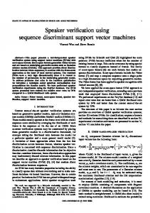
NIST2000_ALL 50 DCF=0.028008 ALL

40 30

Miss probability (in %)

20

10 5

2

0.5

0.1 0.1

0.5

2 5 10 False Alarms probability (in %)

20

30

40

50

Figure 1: DET curve obtained with factor analysis likelihood ratio statistics. The test set is a subset of the NIST 2000 test set containing both electret and carbon data. Male and female trials pooled. DCF = 0.028, EER = 7.2%.

matched with the test set. As we have already explained, we used a subset of the NIST 2000 test set for testing and a disjoint subset of Switchboard II, Phases 1 and 2 for training in these experiments. We used the entire training set to estimate genderdependent GMM’s with 2,048 Gaussians and gender-dependent PCA models with 300 speaker factors and 100 channel factors. We reduced the rank of v(s) to 100 for each target speaker s in evaluating the likelihood ratio statistic (5) and we used 50 tnorm speakers for each test utterance. On the female portion of our test set, the PCA model gave a DCF of 0.030 and an EER of 8.1%. These results can be compared with the results reported in Line 5 of Table 2. The experiment reported in Line 7 of Table 2 showed that it was possible to compensate to some extent for the mismatch between the training and target speaker populations in the experiments on the 1999 data by converting a PCA model to a factor analysis model. By using the same strategy here we were able to obtain a DCF of 0.028 and an EER of 7.5% on the female portion of our test set. So this strategy is effective even if there is no evident mismatch although, as one would expect, the improvement in this case is smaller. Replicating this experiment on the male portion of our test set we obtained a DCF 0.027 and an EER of 6.4%. Pooling the results (using a genderindependent decision threshold) gave a DCF of 0.028 and an EER of 7.2%. The corresponding DET curve is shown in Fig. 1. For comparison, an EER of 17% on the entire 2000 test set was reported in [23] but we have not been able to find any other published results obtained on the 2000 test set without the primary condition restriction. However it is generally recognized that, although it consists entirely of different number trials, the 2000 test set is of about the same degree of difficulty as the 1999 test set and that DCF’s of roughly 0.037 and EER’s of about 10% can be achieved by the methods in [2]. For our purposes, the important thing to note is that we obtained much better results on the 2000 test data than on the 1999 test data and this difference can be attributed to using a training set which is well matched with the test set.

Large speech databases, collected primarily for speech recognition research, are freely available but scarcely any attempt has been made to exploit them for modeling in speaker recognition. This is perhaps surprising since modeling inter-speaker variability in large populations should produce good priors for estimating speaker supervectors; the fact that the Switchboard databases have been collected in such a way that individual speakers are recorded in multiple sessions should make it possible to get a handle on a problem which is of special importance for speaker recognition, namely how to model inter-session variability and channel variability in particular; and the fact that speech data does not have to be transcribed (at least for textindependent speaker recognition) means that many databases which cannot be used for training in speech recognition (such as Switchboard II and Switchboard Cellular, Part I) can still be used for modeling in speaker recognition. The only arguments against using the Switchboard databases as training sets for modeling in speaker recognition seem to be that these databases are not yet sufficiently representative to serve as universal training sets and, since they have all been used by NIST to construct the test sets for the annual speaker verification evaluations, it is difficult to pursue this line of research using standard test sets. Because of the way the Switchboard corpora have been collected, experimenting with a NIST test set in its entirety necessarily entails using a training set which is mismatched with respect to either the target speaker population or the channel effects in the test data. Thus in developing the factor analysis model, we were only able to experiment with properly matched training and test sets by throwing out half of the target speakers in the NIST 2000 evaluation. (We chose the 2000 test set because the number of target speakers was exceptionally large.) The results of these experiments were better than standard methods (handset detection and GMM likelihood ratios) seem to be capable of achieving but it has to be conceded that the set-up was somewhat idealized because the training and test speakers came from the same databases (Switchboard II, Phases 1 and 2) and the results are not as good as our preliminary experiments [7] and the toy experiment in Section 5.2 might suggest. In order to experiment with one of the NIST test sets in its entirety we judged that our best hope was to use the 1999 test set along with Switchboard II, Phases 1 and 2 for training. The mismatch here arises from the fact that the training speakers are from the American Northeast and Midwest and the target speakers from the South. Considering the success of genderdependent factor analysis modeling [7], any mismatch between the training and target speaker populations is likely to be deleterious but it is probably less serious than the CDMA/GSM mismatch we would have encountered had we attempted to train on Switchboard Cellular, Part I and test on the NIST 2002 or 2003 data. Our results on the 1999 test set were as good as those reported in [2] but no better. Perhaps the most interesting thing to note about them is that they were obtained without handset detection. Since we anticipated that the mismatch between the training and target speakers would be a problem, we made several attempts to adapt the hyperparameters in the PCA models to the target speaker population using the enrollment data provided by NIST and the strategy in Section 2.4. These attempts were unsuccessful; on the other hand converting PCA models into factor analysis models either by estimating d on the enrollment data or using standard relevance factors [2] did prove to be effective. This strategy was also effective on the 2000 test data (even though there was no evident mismatch in this case).

Thus it seems that factor analysis likelihood ratios have the potential to perform better than GMM likelihood ratios in speaker verification but the success of this approach depends on the availability of a a training set which is well matched with the test conditions with respect to both the target speaker population and channel effects.

[15] R. Teunen, B. Shahshahani, and L. Heck, “A model-based transformational approach to robust speaker recognition,” in Proc. ICSLP, Beijing, China, Oct. 2000.

7. References

[17] D. Rubin and D. Thayer, “EM algorithms for ML factor analysis,” Psychometrika, vol. 47, pp. 69–76, 1982.

[1] J.-L. Gauvain and C.-H. Lee, “Maximum a posteriori estimation for multivariate Gaussian mixture observations of Markov chains,” IEEE Trans. Speech Audio Processing, vol. 2, pp. 291–298, Apr. 1994.

[18] H. Jiang and L. Deng, “A Bayesian approach to the verification problem: Applications to speaker verification,” IEEE Trans. Speech Audio Processing, vol. 9, no. 8, pp. 874–884, 2001.

[2] D. Reynolds, T. Quatieri, and R. Dunn, “Speaker verification using adapted Gaussian mixture models,” Digital Signal Processing, vol. 10, pp. 19–41, 2000.

[19] P. Kenny, G. Boulianne, P. Ouellet, and P. Dumouchel, “Speaker adaptation using an eigenphone basis,” IEEE Trans. Speech Audio Processing, in press.

[3] A. Rosenberg and F. Soong, “Recent research in automatic speaker recognition,” in Advances in Speech Signal Processing, S. Furui and M. Sondhi, Eds. New York, NY: Marcel Dekker, 1992, ch. 22, pp. 701–738. [4] A. Martin, M. Przybocki, G. Doddington, and D. Reynolds, “The NIST speaker recognition evaluation: Overview, methodology, systems, results, perspectives (1998),” Speech Communication, vol. 31, pp. 225–254, 2000. [5] B. Moghaddam, “Principal manifolds and probabilistic subspaces for visual recognition,” IEEE Trans. Pattern Anal. Machine Intell., vol. 24, no. 6, pp. 780–788, June 2002. [6] P. Kenny, M. Mihoubi, and P. Dumouchel, “New MAP estimators for speaker recognition,” in Proc. Eurospeech, Geneva, Switzerland, Sept. 2003. [7] P. Kenny and P. Dumouchel, “Disentangling speaker and channel effects in speaker verification,” in Proc. ICASSP, Montreal, Canada, May 2004. [8] P. Kenny, G. Boulianne, and P. Dumouchel, “Eigenvoice modeling with sparse training data,” IEEE Trans. Speech Audio Processing, in press. [9] R. Mammone, X. Zhang, and R. Ramachandran, “Robust speaker recognition,” IEEE Signal Processing Mag., vol. 13, pp. 58–71, Sept. 1996. [10] Q. Li, S. Parthasarathy, and A. E. Rosenberg, “A fast algorithm for stochastic matching with application to robust speaker verification,” in Proc. ICASSP, Munich, Germany, Apr. 1997. [11] E. Yu, M.-W. Mak, and S.-Y. Kung. (2002) Speaker verification from coded telephone speech using stochastic feature transformation and handset identification. [Online]. Available: http://www.eie.polyu.edu.hk/ mwmak/papers/pcm2002a.pdf [12] H. Murthy, F. Beaufays, L. Heck, and M. Weintraub, “Robust text-independent speaker verification,” IEEE Trans. Speech Audio Processing, vol. 7, pp. 554–568, 1999. [13] C. Tadj, P. Dumouchel, M. Mihoubi, and P. Ouellet, “Environment adaptation and long term parameters in speaker identification,” in Proc. Eurospeech, Budapest, Hungary, Sept. 1999. [14] W. Chou, “Maximum a posteriori linear regression with elliptically symmetric matrix variate priors,” in Proc. Eurospeech, Budapest, Hungary, Sept. 1999.

[16] D. Reynolds, “Channel robust speaker verification via feature mapping,” in Proc. ICASSP, Hong Kong, China, Apr. 2003.

[20] M. A. Przybocki and A. F. Martin. (2002) NIST’s assessment of text independent speaker recognition performance. [Online]. Available: http://www.nist.gov/speech/publications/papersrc/ cost275.pdf [21] A. Schmidt-Nielsen and T. H. Crystal, “Speaker verification by human listeners: Experiments comparing human and machine performance using the NIST 1998 speaker evaluation data,” Digital Signal Processing, vol. 10, pp. 249–266, Jan. 2000. [22] The ELISA Consortium, “The ELISA systems for the NIST’99 evaluation in speaker detection and tracking,” Digital Signal Processing, vol. 10, pp. 143–153, 2000. [23] R. D. Zilca. Using second order statistics for text independent speaker verification. [Online]. Available: http://www.research.ibm.com/CBG/papers/ ran odyssey2001 paper.pdf