list>), e.g., the third row of the example is represented by the couple (f3g,fa,d, g,ig). Couples also allow the representation of groups of objects and the attributes.
EXTRACTING HIERARCHICAL GRAPHS OF CONCEPTS FROM AN OBJECTS SET : COMPARISON OF TWO METHODS Nicolas ANQUETIL
D�epartement d'informatique et de Recherche Op�erationnelle Universit�e de Mont�eal, C.P. 6128 Succ. centre-ville Montr�eal (Qu�ebec), Canada, H3C 3J7
and Jean VAUCHER
D�epartement d'informatique et de Recherche Op�erationnelle Universit�e de Mont�eal, Montr�eal, Canada
ABSTRACT Understanding something is to discover the important notions it implies, explaining it is mainly to regurgitate these important notions. Computers, with their abilities to rapidly treats large amount of information, has long been expected to do so. Wille's lattice of concepts 14 is a good mean of browsing through a set of objects and the concepts they embed, but for large corpus there are so many concepts that the user get overwhelmed by the amount of information. An other solution is to extract the concepts using a clustering technique 7 , but there are other inconveniences (time complexity of the algorithms, no incremental algorithms). In this article, we present a method that takes advantage of both approaches, starting from a lattice of concepts, it selects the most relevant ones to ease the understanding of the whole data corpus. We will compare the extracted concept set of both method, to underline each one strength and weakness.
1. Introduction Being able to abstract a generalization from a given set of objects is one of the fundamental manifestation of intelligence. In computer science, it has often been achieve through a statistical mean, the clustering : Conceptual Clustering for Machine Learning, automatic creation of thesauri for Information Retrieval , : : : Other researches have underlined the utility of a lattice structure to browse in a space of concepts (Galois lattice , lattice of concepts ). Both techniques (clustering and construction of a lattice) have strength and weakness, hierarchical clustering algorithms are highly time consuming (time complexity O(n ) where n is the number of data) and not incremental which is incompatible with the dynamic type of corpus commonly dealt with. Galois lattices thanks to Godin can be updated in time linear in the number of concepts of the lattice, but they produce so many concepts, that the user gets overwhelmed by the amount of information. On the other hand, we know very little about what really matters, how 7
12
2
2
3
14
good are the concepts extracted, do the constructed graphs really help to understand the object corpus ? After introducing the notion of lattice of concepts (loc) (also known as Galois lattice) and showing how it discovers the concepts embed in an object set, we present a method that select the most relevant concepts of a loc to promote a better understanding of the data corpus, giving a more synthesized point of view on it. It built a new graph that is more general than the loc from which it is extracted. We then propose a method to compare the quality of the extracted concepts of the two methods. Finally, we will present and comment the results of some experiments we made, applying this method.
2. Galois lattices and extraction of concepts Automatic extraction of concepts depends on the representation scheme chosen for the data, because it has a direct impact on the type of concepts that may be discovered. Galois lattices deal with a simple and general data type, object possessing some attributes from a nite set of attributes. The attributes are said to be Boolean, objects either possess them or not. Table 1 gives an example of a corpus of objects. The objects are numbered 1 to 7 and the attributes are the letters a to i. A cross in row x, column y indicates that object x possess attribute y (thus object 5 possess attributes b, e and g). Table 1: Matrix representation for an object corpus example a b c d e f g h i 1 � � � � 2 � � � � 3 � � � � 4 � � � � 5 � � � 6 � � � � 7 � � � � Such data may also be represented by couples (,), e.g., the third row of the example is represented by the couple (f3g,fa,d, g,ig). Couples also allow the representation of groups of objects and the attributes they have in common as for (f1,4g,fc,f,hg). To emphasize the di�erences between an object of the corpus, i.e. a row in the table (or a couple with a singleton as object list), and an object as member of the rst list of a couple, the rst ones will be referred to as input events or simply events. All the possible couples are not of the same interest, some of them present remarkable properties. For example, the couple (f2,3g,fa,g,ig) : there is no other attribute that belongs to all its objects (f2,3g) and there is no other object that possess all its attributes (fa,g,ig). It is said to be a complete couple. (f4,5g,fbg)
is an other complete couple, whereas (f1,2g,fag) is not because it does not include c which also belongs to the objects 1 and 2, neither is (f4g,fc,f,hg) because it lacks the object 1 which also possess the attributes c, f and h. One can de ne a partial order on the set of couples : given two couples C = (O ; A ) and C = (O ; A ), C < C , A � A . Moreover, if C and C are two complete couples, then C < C , A � A , O � O . This partial order can be used to generate a graph which is a Galois lattice : the vertices of the graph are the complete couples, and there is an edge between two vertices C , C i� C < C and there is no other vertex C such that C < C < C . Figure 1 pictured the Galois lattice representation of the example of table 1. 1
1
1
2
2
2
1
1
2
1
1
2
2
1
1
2
2
1
2
2
1
2
3
1
3
2
[1,2,3,4,6,5,7],[]
[4,5,6],[b]
[2,3,5,6,7],[g]
[1,2,3,6],[a]
[2,3,6],[a,g]
[5,6],[b,e,g]
[2,3],[a,g,i]
[6],[a,b,e,g]
[3],[a,d,g,i]
[1,2,4,7],[c]
[1,2],[a,c]
[2,7],[c,g]
[1,4,7],[c,f,h]
[1],[a,c,f,h]
[7],[c,f,g,h]
[4],[b,c,f,h]
[2],[a,c,g,i]
[0,1],[a,b,c]
concept: extent={0,1}; intent={a,b,c}
[],[a,b,c,d,e,f,g,h,i] concept containing an input event vertice linking two concepts
Figure 1: Galois lattice representation for the corpus of table 1 Following Wille's terminology , the complete couples will be referred to as concepts, as they synthesized in their attribute list (the intent of the concept) the information common to all their objects. The object list of a concept is its extent. The partial order < is seen as an inheritance relation between concepts and sub-concepts. The Galois lattice structure will be the lattice of concepts (loc). This terminology is coherent with the mathematical properties shown previously. C < C , A � A states that if C is a sub-concept of C , it must have a longer description (i.e. more attributes). Conversely, C < C , O � O states that C being a specialization of C , it must pertains to less objects. The architecture has proven its utility for browsing purposes , however it has no synthesis capabilities, it usually extracts more concepts than the initial number of events it is given. 14
1
2
1
2
2
1
1
1
2
2
1
2
2
The next section explains how we build a graph of concepts which actually synthesize the data corpus while still allowing some browsing. This technique is based on hierarchical clustering.
3. Extended hierarchy of concepts We have developed an alternative method to build a graph of concepts, which we call extended hierarchy of concepts (ehoc) as it is mainly based on a hierarchical clustering method. We rst introduce the clustering technique and show how it is used to extract concepts, before presenting an original hierarchical clustering algorithm to extract concepts that we call clustering from a lattice. 3.1. Traditional hierarchical clustering
Clustering has long been used to discover the concepts of an event set (Conceptual clustering , ID3 ). Clustering is a statistical mean that aims at gathering into coherent clusters, some set of events. The goal to achieve is to made each event closer to the events of the same cluster than to any other one . 7
11
5
Table 2: Some classical distance measures a b c Jaccard a a b c S�rensen-Dice a a b c d Russel & Rao a a b c d Simple-Matching a d a b c d Rogers-Tanimoto a d ad bc Yule ad?bc + +
2 + + 2
+ + +
+ + + +
+2 +2 + +
Phi
pa
+
b a c b d c d p(aad+?b)(bca+c) a
( + )( + )( + )( + )
Ochiai a : number of common attributes b : number of attributes private to one event c : number of attributes private to the other event d : number of missing attributes in both events Fundamental to clustering methods is the notion of distance, to measure how closer two events are. For events represented as couples, there exist several \classical" distance measures, some of them are listed in table 2 (from ). Basically, events are closer if they have many attributes in common and few which di�ers (attributes 6
private to either objects). All measures essentially divide the number of private attributes by the number of common ones. There are various types of clustering algorithms. For automatic concept discovery, the hierarchical ones are preferred as they produce a hierarchy of concepts which may be viewed as an inheritance tree. One may also use it as a decision tree to identify an event. Moreover, they require no knowledge of the number and type of concepts to be extracted. We will make no di�erence between the bottom-up (agglomerative) and the topdown (divisive) hierarchical clustering algorithms, as they have the same properties. We will solely consider the bottom-up techniques. These algorithms maintain a list of active clusters yet to be processed and result in a binary tree of clusters. They may be sketched as follow : � (Initialization) set each input event as an active atomic cluster � while there is more than one active cluster do { nd the two closest active clusters { create a new cluster as a combination of these two ones, it will be their parent in the nal cluster tree { deactivate the two clusters and activate the new one
end while
Also fundamental to the hierarchical clustering algorithms is the way a new cluster is build from its two sons. To be considered a concept, each new node must be constructed so as to synthesize the attributes of the two nodes it groups together. A common and simple way to do this is to take the union of their objects and the intersection of their attributes (equivalent to the intersection of the objects' attributes). The tree of clusters is a hierarchy of couples, but it still lacks three important properties to t our requirements (having a hierarchical graph of concepts) : � Being a binary tree, it creates an arti cial hierarchy between couples with the same intent but di�erent extents. This occurs when the associated concept has more than two sub-concepts. � Being a tree, it may not fully re ect the inheritance relation between the couples, which usually is a multiple inheritance relation. � Due to these two problems, the couples in the tree may not be complete. Because of the arti cial hierarchy of couples, the sub-couples may lacks some objects in their extent. Because of the simple inheritance constraint, some super-couples, does not \know" all their sons and also lacks some objects in their extent. In we propose a solution to remedy these problems, it builds a general graph of concepts from the binary tree of clusters. This is done in three steps : 1
[1,2,3,4,6,5,7],[]
[2,3,5,6],[g]
[1,4,7],[c,f,h]
[2,3],[a,g,i]
[5,6],[b,e,g]
[5],[b,e,g]
[6],[a,b,e,g]
[3],[a,d,g,i]
[7],[c,f,g,h]
[2],[a,c,g,i]
[1,4],[c,f,h]
[1],[a,c,f,h]
[4],[b,c,f,h]
[1,2,3,4,6,5,7],[]
[2,3,5,6,7],[g]
[1,4,7],[c,f,h]
[0,1],[a,b,c]
cluster: obj. list={0,1}; att. list={a,b,c} cluster containing an input event
[5,6],[b,e,g]
[2,3],[a,g,i] [7],[c,f,g,h]
[1],[a,c,f,h]
[4],[b,c,f,h]
vertice linking two clusters concept grouping some clusters
[6],[a,b,e,g]
[3],[a,d,g,i]
[2],[a,c,g,i]
vertice linking two concepts
Figure 2: ehoc method applied to the example of Table 1
� All the clusters with the same attribute list are joined into one couple. This is
a very simple task as all these couples are gathered in a subtree, the root of it is taken as the representation of the whole subtree. Note that due to the second problem, this couple may still not be complete. We now have a general tree (a hierarchy) of couples. � The inheritance relation is completely represented, by adding the lacking vertices. This give us a graph (an extended hierarchy) of couples. � At this point, each couple knows all its sons. To get complete couples, we update their object list to be the union of all their sons' object lists. We nally obtain a graph of concepts, that we call extended hierarchy of concepts (ehoc). Figure 2 pictures the application of this method to the example given in table 1. The binary tree of clusters is drawn with plain lines. Clusters circled by a dashed line are to be gathered in one concept (step 1). The dashed edge between two concepts is an added vertice to complete the inheritance relation (step 2). The resulting ehoc is shown in the lower left box. This method actually achieves an abstraction of the data corpus and still allows some browsing through the input events and their super-concepts. However, it is not incremental, thus adding one event to the corpus imposes to recompute the whole
graph. We now present a method that takes advantage of the informations contained in the loc to build an ehoc similar to the one we just obtained, but with a better time complexity. 3.2. \Clustering from a lattice" algorithm
The ehoc extracts a subset of all the concepts contained in the corpus. It selects some of them and discards other ones, which means discarding the information they contains, information which is not important given this particular corpus. However the corpus may (and often will) evolve, some events may be added which would made this lost information needful. The only way to recover this information is to recompute everything. The method is said not to be incremental. This is a serious drawback as the time complexity of the clustering algorithm (thus the minimum time complexity of the whole method) is O(n ) (where n is the size of the corpus). The loc contains all the concepts of the corpus whereas the ehoc selects some of them. It may be considered as a pruned version of the loc. We could use the loc as a starting point to build the ehoc, by selecting some of its concepts instead of extracting them from the corpus. The problem is to select the most relevant concepts. The rst (unsuccessful) experiments we conducted consisted in de ning various measures on each concept, such as the average distance between two events of a concept. We also tried to consider the concepts and events as vectors in the attributes space and compare between them, etc. But the results were not satisfactory, the selected concepts did not formed a good generalization of the corpus. It appeared to us that whereas these unsuccessful experiments consider only one concept at a time, trying to decide if it is important or not, the hierarchical clustering method previously described, gains its e�ciency by comparing each concept to all the others. We concluded that the solution could not be achieved by local methods and that we were to use something more global. On the other hand one of the drawback of the clustering method is its quadratic time complexity, a direct consequence of this global approach. The clustering algorithm compute the distance between each pair of clusters to nd the two closest. The solution we propose is to take advantage of the loc to de ne the neighborhood of a concept prior to compute any distance from it. The idea is that a concept in the loc shares more attributes with its brothers (other sub-concepts of one of its parents) than with any other concepts. On the other hand the more attributes two objects share, the closer they should be according to the \classical" distance measures (see previous section). Thus each concepts should be closer to its brothers than to any other concepts. The solution consists in clustering the concepts of the loc according to the following algorithm, mostly based on the one exposed before (classical hierarchical clustering algorithm) : � (Initialization) set as active, each concept of the loc that contains one or more events from the input corpus 2
� while there is more than one active concept do { nd the two closest neighbors active concepts { nd the common parent of the two concepts { deactivate the two concepts and activate their parent end while
This basic algorithm needs to be re ned to deal with two \pathologic" cases : � The neighborhood of a concept may enclose not only its brothers, but also its parents. In this case, the parent will certainly be the closest concept to its son and, soon or later, they will be selected, the third step of the loop (deactivating the two concepts and activating the new one) will then resume into deactivating the son and keep the parent activated. � Due to the sequential progress of the algorithm, it may happened that a node with very few and far brothers cannot be joined to any of them because they are not active anymore. In this case we have to enlarge the notion of neighborhood to the cousins, i.e. descendents of one of the node's grandparents. If those ones have already been deactivated, we have to enlarge further to the greatgrandparents and so on. The clustering from a lattice algorithm builds a hierarchy (general tree) of concepts. To get an ehoc, we still need to fully re ect the inheritance relation between the concepts as already done for the binary tree of clusters. The hierarchy of concepts resulting of the clustering from the loc for our example is given in gure 3, compare it to the original loc ( gure 1) and to the graph obtained from the traditional hierarchical clustering method ( gure 2). For the sake of clarity, the inheritance relation between the concepts has not been fully represented. The gure only pictures the result of the clustering form a lattice algorithm, and not the ehoc. We have presented so far two methods to extract a hierarchical graph of concepts from a set of events. We may now ask how they compares, and which one (if any) is the best.
4. Comparison of the methods Although the two methods we have presented (loc and ehoc) produce graphs of concepts, they are not appropriately compared as simple graphs. Two reasons made us only consider the vertice (concept) sets of the graphs and discarding their edge (inheritance relation) sets : � The edges of the graphs can be completely deduced from their vertices. It turns out to stress the importance of the vertices which quality in uence that of the edges,
[1,2,3,4,6,5,7],[]
[4,5,6],[b]
[2,3,5,6,7],[g]
[1,2,3,6],[a]
[2,3,6],[a,g]
[5,6],[b,e,g]
[1,2],[a,c]
[2,3],[a,g,i]
[6],[a,b,e,g]
[3],[a,d,g,i]
[1,2,4,7],[c]
[1],[a,c,f,h]
[2,7],[c,g]
[7],[c,f,g,h]
[1,4,7],[c,f,h]
[4],[b,c,f,h]
[2],[a,c,g,i]
[],[a,b,c,d,e,f,g,h,i]
[0,1],[a,b,c]
selected concept
[0,1],[a,b,c]
discarded concept concept containing an initial data vertice linking two selected concepts vertice incident to a discarded concept
Figure 3: Clustering from the loc of table 1 example
� When comparing two theories (concept sets), you are only concerned by how
well they explain the world, and do not care which concepts are specializations of other ones. First, we observed from a few examples that the loc, extracted much more concepts than the ehoc. A loc commonly has 2 times more additional concepts than input events, in examples up to 6.7 times more additional concepts are given. In its example, Wille extracts 47 new concepts from a corpus of 18 objects, which makes 2.6 times more additional concepts. This means that the loc often extracts two (and more) concepts for each event it is given. This really seems a lot, and we may ask ourselves how relevant most of the concepts are. Comparatively, while testing the ehoc, we have never experienced a number of additional concept more than half the number of input events. With Wille example, we extracted only 8 new concepts, 0.4 times the number of objects. It means than in average, the ehoc extract one new concept for each two events it is given. We will show latter that the actual limit is one time more additional concepts. However, the fact that the ehoc commonly extracts four times less concepts than the loc is not very interesting, what we need to know is \are these concepts relevant to the event set ?" This is the question this section tries to answer. 3
14
4.1. Recall, precision and the lawyer's approach
Calling E the concept set extracted by some method, El will be the set of concepts extracted by Wille's method (l for lattice) and Eeh will be the set extracted by the ehoc. These sets of extracted concepts will be compared to A the set of actual concepts in the corpus. Let us state rst that we are well aware of the \fuzzy" nature of A, two people, given the same event corpus will certainly not give the same de nition (in extension) to A, because each one have its own prede ned set of concepts extracted from a much larger corpus, namely the real word. However it is reasonable to consider that any group of people will agree on a good de nition of A. We know very little on A in theory, given a set D of events (or data) taking their attributes (or properties) from a set P , the theoretic upper bound for kAk is min(2kDk; 2kPk) (as concept are couples of subsets of D and P ). In , Godin shows that in practical cases, when there is a xed upper bound on the number of attributes of an event, the number of concepts in the corpus is linearly bounded with respect to kDk. A practical upper bound on kAk is kkDk, where k is the average number of attributes of an event. As it extracts all the concepts of the corpus, the loc exhibits the same upper bound as A. For kElk, the theoretic upper bound is min(2kDk; 2kPk) and the practical upper bound kkDk. Finally for the ehoc a concept being the combination of at least two other ones, the upper bound is reached when the graph is a binary tree, having kDk events (\atomic concepts") and kDk ? 1 inner (extracted) concepts, which makes an upper bound for kEg k = 2kDk (lets forget the '?1' constant). Having stated these bounds, we can try to compare the various concept sets. We are obviously looking for a method which gives us E = A, i.e. for which all the extracted concepts are actual concepts and which do not \miss" any actual concept. Information Retrieval (IR) experiences similar problems, given a document database, it must extract the documents relevant to a query. In IR, the e�ciency of a method is quanti ed by two measures ; recall is the percentage of relevant documents in the database that the system nd ; precision is the percentage of relevant documents among the ones retrieved by the system. A recall of 100% is easily achieved by retrieving all the database, but the precision will be very poor. Conversely, by retrieving very few documents (say one) the precision rate is almost certain to be very high (either 100% or 0% in fact), but the recall will be equally low. One can see the two methods we are studying as IR systems that work on a virtual database, the set of all existing concepts. A query is composed of all the events of the corpus, against which the documents (concepts) are matched. Each concept is a document relevant or not to the query the system is given, A is the set of relevant documents. The e�ciency of the concept extraction methods may be quanti ed by the two measures recall and precision. We have already said that the loc extract all the possible concepts in the event set it is given, this corresponds to an IR system which would retrieve all the database 3
to answer a query, its recall rate is 100%. However we will show that the precision is usually not as good (its actual value is : kkEAlkk ). Having a recall rate of 100%, the method may be said to be complete, a method which would achieve a precision rate of 100%, could be said to be sound, this is not the case for the loc. The ehoc is not complete, its kEg k upper bound of 2kDk is too far from the kAk upper bound of kkDk. Just think to events being texts, when k, the average number of attributes (here words), could be hundreds or thousands. However, clustering is a statistical mean intended to extract relevant clusters of events from a possibly noisy corpus, which allow us to assert that the ehoc has a very high precision rate. We will show that most of the time, its precision rate is 100%, still, for extremely noisy corpus, the method will extract \wrong" concepts in the sense that an expert of the domain will not have accepted them. But once more, what made the expert so e�cient is that his corpus is much larger than the event set he is considering. The problem is, from which point does noise becomes data ?kEAssuming a 100% precision rate for the ehoc, its recall rate could be evaluated to kAehkk . Due to the imprecision on the set kAk, and the statistical characteristics of the ehoc, we will not dare call it sound, we propose to say statistically sound. The question \which of the two methods is the best ?" becomes : \Should a method promote the recall or the precision ?", \Should it be complete or (statistically) sound ?" Sound methods will usually be preferred to complete ones, because understanding something is being able to reduce it to its signi cant properties, rather than making an extensive list of all the properties you ever heard about to make sure you do not miss any. In IR, depending on the application, one wants to promote one or the other measure. When searching through a case database, lawyers wants a hight recall rate, because they must not miss a case which could help them. On the other hand, while searching for references in a publication database, one needs a good precision to avoid reading irrelevant papers while worthy papers may be reached by other means (cross referencing). The loc use the lawyer's approach, it have a perfect recall rate because it retrieves all the database, but of course its precision may be very poor. Conversely, the ehoc promotes the precision at the expense of the recall. Leaving out this discussion, the next section presents an actual measurement of precision and recall for both method. 4.2. Measuring Recall and Precision
We said that recall and precision could not be actually measured due to the lack of information on set A. In this section we present an experiment which bypass this di�culty. To measure the recall and precision of both methods, we have designed an example (our world) for which A is known. The events take their attributes from various
facets , each facet being a hierarchy of attributes. The event corpus was generated by randomly selecting an attribute in each facet for a given number of objects. We then applied both methods to the corpus and compare the results. For each experiment, the A set was calculated using the loc. We computed the intersection of the loc's set of concepts (known to be exhaustive for the given corpus) and our world's set of concepts. We then could measure the recall and precision of the methods in regard to A. We conducted three series of experiments : � generation of \perfect" (without noise) sets of events of various size. Our world has 114 possible di�erent attribute lists, the corpus' sizes are expressed in this unit. A corpus of size 1 has 114 objects, one of size 20 has 2850. For each size, we conducted 10 experiments. The recall and the precision for a size are the average value of the 10 experiments. � introduction of noise in a corpus of more than 1000 events (size 10 = 1140 events). Noise is de ned to be the insertion of extraneous attributes which do not appears in the normal facets. A small event corpus rarely contains all the possible concepts of our world. That occurs with high probability only for large corpus (at least size 20). To keep the experiments su�ciently short and still have enough concepts in the corpus, we limited ourselves to size 10. Noise was introduce with probabilities, ranked from 0.1 (10%) to 1 (100%), with steps 0.1 . For each noise probability, we made 10 experiments. � introduction of errors in a corpus of size 10, errors being de ned to be either the insertion or deletion of a normal attribute to an object's description. To be consistent with real world event corpus, error probability should be far much lower than the noise probability we just gave. We rst ranked it from 0.01 to 0.1, but the results proved both method resistant enough to increase it. The results given further have been obtained with error probabilities ranking from 0.1 to 1 (steps 0.1). For all the experiments, we only considered the sets of extracted concepts, omitting the events themselves. Although this can be subject to discussion for the perfect events corpus, it avoid perturbing twice the results with noisy/erroneous events and noisy/erroneous extracted concepts. We now present and comment the results of these experiments. 10
4.2.1. First series of experiments (perfect events corpus) Figure 4 summarize the result of the rst series of experiments for the loc (left) and the ehoc (right).
Lattice of Concepts
Extended Hierarchy of Concepts recall precision
100
80
percentage
80
percentage
recall precision
100
60
60
40
40
20
20 1x
5x
10x
15x 20x corpus size
25x
30x
22.8
1x
25.1
24.9
5x
10x
26.1
25.1
24.2
15x 20x corpus size
25x
27.2
30x
Figure 4: Recall and Precision for perfect events corpus Unsurprisingly, the recall of the loc is 100%, it could not have been otherwise as, for perfect event corpus, the A set (our reference) is the set of concepts extracted by the loc. For both method, the precision is also 100%. As there is neither noise, nor error, the corpus contains only valid concepts. As expected, ehoc's recall is far lower, due to the upper bound on the number of concepts extracted. This must not be misunderstood as a proof of its ine�ciency. First, because explaining a theory (a set of concepts) by giving all its concepts is not a good idea. One better teach it by choosing some of the concepts and make sure they are well understood before exposing some other. That's what the ehoc allows to do. Second, because we are considering perfect event corpus, which seldom occurs in real world. Examining the number of extracted concepts ( gure 5) brings a surprise. Lattice of Concepts # of concepts # of extracted concepts
250
# of concepts # of extracted concepts
250
200
number of concepts
number of concepts
Lattice of Concepts
150 100 50
200 150 100 50
0
0 1x
5x
10x
15x 20x corpus size
25x
30x
1x
5x
10x
15x 20x corpus size
25x
30x
Figure 5: Number of extracted concepts for perfect events corpus Figure 5 tends to prove that, for ehoc, there is a correlation between the number of actual concepts in the corpus and the number of extracted concepts. However, we
said in a previous section that the upper bound on the number of extracted concepts depends on the corpus size. We expected an increase of the precision linear to the augmentation of the number of events. We explain this abnormality by a shadowing e�ect, a kind of local minima. When a concept has been extracted from two events, it exerts a strong attraction on all the events belonging to it, thus shadowing the other concepts these events belongs to. We soon will see another unexpected consequence of the shadowing e�ect. 4.2.2. Second series of experiments (noisy events corpus) Lattice of Concepts
Extended Hierarchy of Concepts
120
120 recall precision
100
recall precision 100 99.8 100 99.8 99.4 99.2 97.9 97.7 94.7
100
84.6 80
percentage
percentage
80 66.8 60 45.5 40
44.6
40
35.4 29.1
20
60
24.2 21.6 20.4
18.9 18.5 19.6
0
20 24.9 25.5 25.0 26.124.4
30.3 26.3 27.2 27.7
34.7
0 0
0.1 0.2 0.3 0.4 0.5 0.6 0.7 0.8 0.9 noise probability
1
0
0.1 0.2 0.3 0.4 0.5 0.6 0.7 0.8 0.9 noise probability
1
Figure 6: Recall and Precision for noisy events corpus The second series of experiment plainly con rms what we expected, and exposed in the previous section : � loc's recall remains 100% (for the reason previously explained), whereas its precision decreases abruptly with increasing noise probability. � the precision of the ehoc stays high even for an extremely (but not abnormal) noisy corpus. � An unexpected consequence of noise introduction is the increase of the ehoc's recall. We suspect that the presence of noise introduces perturbations that breaks down the shadowing e�ect. This could be compare to the random moves of simulated annealing used in Operational Research to avoid falling into local minimas. Recall really takes o� when the precision begins to decrease (noise probability > 0:7). At this step, the large proportion of noise causes noisy concepts to be extracted at rst. The noise is quickly pushed aside in the succeeding steps (and succeeding extracted concepts), however it had allowed some concepts which would have been shadowed to emerge. More simply, gure 6 shows that from a 50% noise probability, the loc extract more than 3 \false" concepts for each \good" one (for 70% noise probability, this
raises to 4 errors for each success). On the contrary, the ehoc does not extract all the good concepts, but almost all the concepts it extracts are relevant. This is even more obvious in gure 9 which gives the number of extracted concepts. Lattice of Concepts # of extracted concepts # of actual concepts extracted
1800
1600
1400
1400
1200 1000 800 600
# of extracted concepts # of actual concepts extracted
1800
1600
number of concepts
number of concepts
Extended Hierarchy of Concepts
1200 1000 800 600
400
400
200
200
0
0 0
0.1 0.2 0.3 0.4 0.5 0.6 0.7 0.8 0.9 noise probability
1
0
0.1 0.2 0.3 0.4 0.5 0.6 0.7 0.8 0.9 noise probability
1
Figure 7: Number of extracted concepts for noisy events corpus Figure 9 shows that for the loc, the number of extracted concepts increases linearly with the amount of noise, whereas the number of actual extracted concepts remains constant. Introduction of noise produces new concepts, but they are not relevant. This is where the loc reveals its major weakness, it does not make any di�erence between all these concepts. 4.2.3. Third series of experiments (erroneous events corpus) Results of the third series of experiments are given in gures 8 and 9. Lattice of Concepts recall precision
100 80.7
80
65.7 60
55.1 49.5 42.4 39.4
40
35.3 34.2
recall precision 99.6 99.2 99.1 98.8 97.8
100
percentage
percentage
Extended Hierarchy of Concepts
80 60 40
30.9 28.9
20
24.9 23.4 17.3 16.3
20
0
0.1 0.2 0.3 0.4 0.5 0.6 0.7 0.8 0.9 error probability
1
0
12.9 13.5 11.2 10.5 10.1
8.9 8.9
0.1 0.2 0.3 0.4 0.5 0.6 0.7 0.8 0.9 error probability
1
Figure 8: Recall and Precision for erroneous events corpus For the loc, the experimentation with errors gives results similar to the previous one. The loc extracting all the concepts of a corpus, it is more resistant to deletion of actual attributes than to insertion of noise. Remember that errors are either insertion
or deletion of attributes, thus for an error probability of 100%, perturbations are introduced with a probability of only 50%. This is why, the precision rate of the loc is higher than in the previous series of experiments. The third series of experiments seems to proves a major failure of the ehoc's recall, but one must not forget that we rst experienced lower errors probabilities (from 1% to 10%). We choose these hight errors probabilities only to enlighten the behavior of both methods when exposed to erroneous corpus. Despite the growing proportion of erroneous concepts in the corpus ( gure 9), the ehoc's precision stays almost perfect. The price too pay is a poor recall, which decreases throughout the experiment. Unlike noise, errors does not helps to break down the shadowing e�ect. On the contrary, deletion of attributes introduces events in the corpus that are considered as generalizations of other (unmodi ed) events. These already present concepts reinforce the shadowing e�ect. Lattice of Concepts 800
# of extracted concepts # of actual concepts extracted
700 600 500 400 300
600 500 400 300
200
200
100
100
0
# of extracted concepts # of actual concepts extracted
700
number of concepts
number of concepts
Extended Hierarchy of Concepts 800
0 0
0.1 0.2 0.3 0.4 0.5 0.6 0.7 0.8 0.9 error probability
1
0
0.1 0.2 0.3 0.4 0.5 0.6 0.7 0.8 0.9 error probability
1
Figure 9: Number of extracted concepts for erroneous events corpus 4.2.4. Experiments summary All our experiments boil down to the following conclusions : � As expected, the loc promotes the recall at the expense of the precision (the lawyers' approach). It makes no di�erences between noisy/erroneous concepts and actual concepts. � On the contrary, the ehoc tries to \explain" the corpus by retrieving only actual concepts and discarding not only noisy/erroneous concepts, but also actual concepts that are not important. There is one more thing that the experiments could not show but that we may deduce. Even for a perfect corpus, the loc still extracts too much concepts. Considering all concepts on an equal footing, it does not explain the corpus, in the sense that it does not give a synthesized view of it. On the contrary, the ehoc made a
selection on the concept set. It gives an explanation of the corpus, which may not be the one we would have favored, but which could be used as a starting point.
5. Utility of these methods Objects' attributes in the data representation scheme of section 2 are atomic. However, the de nition of loc we gave, may be generalized to handle more complex data representation schema. 5.1. Extending the data representation scheme
First, we may want to allow attributes to have values, what we call multi-valued attributes. In that case, we expect the classi cation in the graph of concepts to be made on the attributes as well as their values. Given a couple Ci, we used to note its object list Oi and its description (attribute list) Ai. Each member of Ai, now an attribute/value pair, will be noted ai;j : vi;j . To incorporate some data in a loc, we need a generalization relation to be de ned on the objects' descriptions. When objects' descriptions are vectors of boolean attributes as in the previous sections, a description (an attribute list) A is said to be more general than a description A i� A � A . For multi-valued attributes, we will said that the concept C is more general than the concept C (C < C ) i� 8a ;i 2 A (i.e. a ;i has a value), 9a ;j 2 A : 1. a ;i and a ;j are the same attribute, and, 2. v ;i is more general than v ;j . Which means that C is more general than C if all the attributes of C are also attributes of C , and these attributes' value are more general for C than for C . 1
2
1
2
1
1
2
2
1
1
2
1
1
2
2
1
2
1
2
1
2
1
O1 :
elephant
has
trunk
length
2
1.50 m.
Figure 10: Example of relations between objects The data representation scheme may be further extend to accept relation between objects. A relation may be seen as an object whose attributes (the roles of the relation) have other objects for values. To avoid confusion, we will call an object constituted of several related objects, a composite object. Consider the example of gure 10, there are two composite objects (the two graphs). The rst composite object, O , contains : � three objects o ; = elephant and o ; = trunk that may have attributes (not shown here) and o ; = 1.50 m that may be considered a value as well as an object with no attributes. 1
11
12
13
� two relations r ; = has (with two roles, the possessor and the possessed) and 11
r ; = length (with two roles also, the object measured, and the measure). Before de ning a generalization relation between composite objects, we will extend the above de nition of a generalization relation for objects with multi-valued attributes to take into account the new notion of relation. A relation r will be more general than a relation r i� r have all the roles of r , and, the roles' objects for r are more general (following the previous de nition) than the corresponding roles' objects for r . The two de nitions are very much alike, the roles being attributes and the roles' objects being attributes' values. Finally we will said that a composite object O will be more general than a composite object O i� O have all O 's relations, and that these relations are more general (following the previous de nition) for O than for O . Lets us state, that following the multi-attributes generalization relation, the object mammal is more general than the object elephant, and the object nose more general than the object trunk, we may then say that the composite object O of our example is more general than the composite object O , because : 1. O has all O 's relations (i.e. the relation has), and, 2. the relation has in O is more general than the relation has in O , following the above de nition. 12
1
2
2
1
1
2
1
2
2
1
1
2
2
1
2
1
2
1
5.2. Conceptual graphs and graphs of concepts
These three de nitions of generalization relations allow composite objects to be incorporated in a loc. The reader may have notice that what we call composite objects are also conceptual graphs (Sowa ). Conceptual Graphs have been widely used and studied since 1984. Mineau proposes to structure a set of such graphs in a Knowledge Space, which ends to be another pruned version of the loc. Mineau only consider a restricted version of the conceptual graphs. The constrains he sets ensure that the graphs can be decomposed without ambiguity into a set of triplet . Before building his graph, Mineau generates all the \canonical" generalizations of the triplets (which we will call basic triplet from now on). A \canonical" generalization being a triplet where at least one of the elements have been replaced by a wildcard \?". For example, our rst composite object O may be represented by the two basic triplets and and the set of \canonical" generalization for the rst basic triplet will be f, , , g. The \canonical" generalizations are incorporated in the Knowledge Space along with the basic triplets. The Knowledge Space may then select the \canonical" generalizations that are common to several basic triplets. This structure allows the system to answer quickly to questions as \Who has a trunk ?"