particular, for reading blood glucose level from subcutaneous electric current .... is fixed, one may follow [17] and select a kernel by minimizing the Tikhonov ...
EXTRAPOLATION IN VARIABLE RKHSs WITH APPLICATION TO THE BLOOD GLUCOSE READING VALERIYA NAUMOVA, SERGEI V. PEREVERZYEV AND SIVANANTHAN SAMPATH Abstract. In this paper we present a new scheme of a kernel adaptive regularization algorithm, where the kernel and the regularization parameter are adaptively chosen within regularization procedure. The construction of such fully adaptive regularization algorithm is motivated by the problem of reading the blood glucose concentration of diabetic patients. We describe how proposed scheme can be used for this purpose and report the results of numerical experiments with real clinical data.
1. Introduction In this paper we consider the problem of a reconstruction of a real-valued function f : X → R, X ⊂ Rd , from a given data set z = {(xi , yi )}ni=1 ⊂ X × R, where it is assumed that yi = f (xi ) + ξi , and ξi = {ξi }ni=1 is a noise vector. At this point it should be noted that the reconstruction problem can be considered in two aspects. One aspect is to evaluate the value of a function f (x) for x ∈ co{xi }. It is sometimes called as interpolation. The other aspect is to predict the value of f (x) for x ∈ / co{xi }, which is known as extrapolation. In both aspects the reconstruction problem is ill-posed, and the task of solving it makes sense only when placed in an appropriate framework. The numerical treatment of ill-posed problems with noisy data requires the application of special regularization methods. The most popular among them is the Tikhonov method, which in the present context consists in constructing a regularized solution fλ (x) as a minimizer of the functional |z|
1 X (yi − f (xi ))2 + λ||f ||2W2r , Tλ,r (f ) = |z| i=1
(1)
where |z| is the cardinality of the set z, i.e. |z| = n, and λ is a regularization parameter, which trades off data error with smoothness measured in terms of a Sobolev space W2r [21]. The Tikhonov method, even in its simplest form (1), raises two issues that should be clarified before use of this scheme. One of them is how to choose a regularized parameter λ. This problem has been extensively discussed. A few selected references from the literature are [20, 6, 5, 13]. Another issue which needs to be addressed is the one of the choice of a space, which norm is used for a penalization. The impact of the chosen norm is most explicit in Tikhonov
2 V. Naumova, S. V. Pereverzyev and S. Sivananthan regularization [7]. Moreover, the choice of the proper space is firmly connected to the problem of choosing a representation of the output fλ (x). Thus, the choice can make a significant difference in practice. Despite its significance, the second issue is much less studied. Note there are still no general principles to advise a choice and only in a few papers [21, 17, 15, 6] some methods for finding an appropriate space for the regularization of ill-posed problems have been proposed. Keeping in mind that a Sobolev space W2r used in (1) is a particular example of a Reproducing Kernel Hilbert Space (RKHS), the above mentioned issue is, in fact, about the choice of a kernel for an RKHS. Exactly in this context this issue has been studied recently in [17], but, as it will be seen from our discussion below, the kernel choice suggested in [17] does not fit well for extrapolation. With this application in mind, we will propose another kernel choice rule (kernel adaptive regularization algorithm – KARalgorithm), which is based on a splitting of a given data set z, oriented towards extrapolation. The article is organized in the following way. In section 2 we outline a theoretical background about RKHS, present our kernel choice criteria, and prove the existence of the kernel that satisfies it. We also illustrate our approach by a few academic examples. In section 3 we discuss a possibility to use the proposed approach in diabetes therapy management, in particular, for reading blood glucose level from subcutaneous electric current measurements and report the results of numerical experiments.
2. Regularized interpolation and extrapolation in RKHS 2.1. Reproducing Kernel Hilbert space A Reproducing Kernel Hilbert space H is a space of real-valued functions f defined on X ⊂ Rd such that for every x ∈ X the point-wise evaluation functional Lx (f ) := f (x) is continuous in the topology induced by the inner product h·, ·i , which generates the norm of H. By the Riesz representation theorem, to every RKHS H there corresponds a unique symmetric positive definite function K : X × X → R, called the reproducing kernel of H = HK , that has the following reproducing property: f (x) = hf (·), K(·, x)i for every x ∈ X and f ∈ HK . For any positive definite function K(x, y) on X there exists a uniquely determined Hilbert space H = HK with an inner product h·, ·i, admitting the reproducing property. Conversely, each RKHS H admits a unique reproducing kernel K(x, y). A comprehensive theory of Reproducing Kernel Hilbert spaces can be found in [1]. In the sequel we will deal with the situation when X is a compact in Rd . Then, it is known [23] that HK is continuously embedded in the space of continuous functions C(X), as well as in the space L2 (X) of functions, which are square-summable on X. Moreover, the canonical embedding operator JK : HK → L2 (X) is compact. Now we can write the problem of a reconstruction of f ∈ HK from noisy data z in the form JK f = f ξ , (2) where fξ ∈ L2 (X) and is such that fξ (xi ) = yi , i = 1, 2, . . . , |z| . Note that in general, fξ ∈ / Range(JK ), and the problem (2) is ill-posed. Moreover, noisy data z allow the access only to a discretized version of (2), that can be written as follows: Sx f = y,
(3)
Extrapolation in variable RKHSs with application to the BG reading |z|
3
|z|
where x = {xi }i=1 , y = {yi }i=1 and Sx : HK → R|z| is the sampling operator Sx f = |z| {f (xi )}i=1 . Observe that the problem (3) inherits the ill-posedness of (2) and should be treated by means of a regularization technique. If a kernel K has been already chosen, several methods of the general regularization theory can be applied to the equation (3), as it has been analyzed in [2]. In particular, as we stated in the Introduction, one can apply the Tikhonov regularization. In this case the regularization estimator / predictor fλ (x) = fλ (x; K, z) is constructed from (3) as the minimizer of the functional |z|
1 X Tλ (f ) = Tλ (f, K, z) = (yi − f (xi ))2 + λ||f ||2K , |z| i=1
(4)
where || · ||K is a standard norm in an RKHS HK . From the Representer Theorem [21] it follows that the minimizer of (4) has the form fλ (x; K, z) =
|z| X
cλi K(x, xi ),
(5)
i=1
− where a real vector → cλ = (cλ1 , cλ2 , ..., cλ|z| ) of coefficients is defined as follows → − → y, cλ = (λ|z|I + K)−1 − |z|
here I is the unit matrix of the size |z| × |z|, K = {K(xi , xj )}i,j=1 is the Gram matrix, and → − y = (y1 , y2 , ..., y|z| ). 2.2. Adaptive parameter choice When a kernel K is already chosen, an appropriate choice of the regularization parameter λ is crucial to ensure a good performance of the method. For example, one can use a data-driven method for choosing the regularization parameter known as the quasi-optimality criterion. It was proposed long time ago in [20], and as it has been proven recently in [13], using this criterion one potentially may achieve an accuracy of optimal order (for a given kernel K). To apply the quasi-optimality criterion one needs to calculate the approximations fλ (x; K, z) given by (5) for λ from a finite part of a geometric sequence Λνq = {λs : λs = λ0 q s , s = 0, ν}, q > 1.
(6)
Then one needs to calculate the norm 2 σH (s) = ||fλs (x; K, z) − fλs−1 (x; K, z)||2K K
:=
|z| |z| X X
λ
(7)
λ
(cλi s − ci s−1 )(cλj s − cj s−1 )K(xi , xj ),
i=1 j=1
and find 2 λ+ = λp : p = arg min{σH (s), s = 0, ν}. K
(8)
4 V. Naumova, S. V. Pereverzyev and S. Sivananthan 2.3. The choice of the kernel from a parameterized set But it seems to be that in practice one of the most delicate and challenging issues is the choice of the kernel K. On the one hand, special cases of the single fixed kernel K have been considered in the literature [9], [5]. On the other hand, in practice we would like to have multiple kernels or parameterizations of kernels to scale well the solution to the problem of interest. This is desirable because then we can choose K from the available set of kernels, dependent on the input data and problem, and get good performing results. Lanckriet et al. were among the first to emphasize the need to consider the multiple kernels or parameterizations of kernels, and not a single a priori fixed kernel, since practical problems often involve multiple, heterogeneous data sources. In their work [15] the authors consider the set m X K({Ki }) = {K = βi Ki } i=1
of linear combinations of some prescribed kernels {Ki }m i=1 and propose different criteria to select the kernel from it. It is worthy of notice that for some practical applications such a set of admissible kernels is not rich enough. Therefore, more general parameterizations are also of interest. Let us consider the set K(X) of all kernels (continuous, symmetric positive definite functions) defined on X ⊂ Rd . Let also Ω be a compact metric space and G : Ω → K(X) be an injection such that for any x1 , x2 ∈ X, w ∈ Ω the function w → G(w)(x1 , x2 ) is a continuous map from Ω to R, here G(w)(x1 , x2 ) is the value of the kernel G(w) ∈ K(X) at (x1 , x2 ) ∈ X × X. Each such a mapping G determines a set of kernels K(Ω, G) = {K : K = G(w), K ∈ K(X), w ∈ Ω} parameterized by elements of Ω. In contrast to K({Ki }), K(Ω, G) may be a non-linear manifold. Example Consider Ω = [a, b]3 , 0 < a < b, (α, β, γ) ∈ [a, b]3 , and define a mapping G : (α, β, γ) → 2 (x1 x2 )α + βe−γ(x1 −x2 ) , where x1 , x2 ∈ X ⊂ (0, ∞). It is easy to see that G(α, β, γ) is a positive definite as the sum of two positive definite functions of (x1 , x2 ). Moreover, for any fixed x1 , x2 ∈ X ⊂ (0, ∞) the value G(α, β, γ)(x1 , x2 ) continuously depends on (α, β, γ). Thus, kernels from the set 2
K(Ω, G) = {K : K(x1 , x2 ) = (x1 x2 )α + βe−γ(x1 −x2 ) , (α, β, γ) ∈ [a, b]3 }. are parameterized by points of Ω = [a, b]3 in the sense described above. Once the set of kernels is fixed, one may follow [17] and select a kernel by minimizing the Tikhonov regularization functional (4) such that Kopt = arg min{Tλ (fλ (·; K, z); K, z), K ∈ K(Ω, G)}. Thus, the idea of [17] is to recover the kernel K generating the space HK , where the unknown function of interest lives, from given data, and then use this kernel for constructing the approximant fλ (·; K).
5
Extrapolation in variable RKHSs with application to the BG reading
To illustrate that such an approach may fail in a prediction of the extrapolation type we 4π π 3π 2 2 2 use the same example as in [17], where f (x) = 0.1(x + 2(e−8( 3 −x) − e−8( 2 −x) − e−8( 2 −x) )), πi and the given set z = {(xi , yi )}14 i=1 consists of points xi = 10 , i = 1, 2, . . . , 14 and yi = f (xi ) + ξi , where ξi are random values sampled uniformly in the interval [−0.02, 0.02]. Note that in [17] the target function f has been chosen in such a way that it belongs to the RKHS 2 generated by the “ideal” kernel Kopt (x1 , x2 ) = x1 x2 + e−8(x1 −x2 ) . The performance of the approximant fλ (x; Kopt , z) with the best λ is shown in the Figure 1. This figure illustrates π 14π , 10 ] the value of f (x) is well-estimated by fλ (x; Kopt , z), while for that for x ∈ co{xi } = [ 10 x∈ / co{xi } the performance of the approximant based on the Kopt is rather poor. Observe that the Figure 1 displays the performance of the approximation (5) with the best λ. It means that the choice of the regularization parameter λ cannot improve the performance of the approximation (4), (5) given by the “ideal” kernel, that is, the kernel Kopt (x1 , x2 ) = 2 x1 x2 + e−8(x1 −x2 ) used to generate the target function f . 0.6
0.5
0.4
0.3
0.2
0.1
0
0.5
1
1.5
2
2.5
3
3.5
4
4.5
5
5.5
Figure 1: The performance of the approximant fλ (x; K, z) (red line) based on the kernel 2 K(x1 , x2 ) = x1 x2 + e−8(x1 −x2 ) generating the target function f . The Figure 2 displays the performance of the approximation (5) constructed for the same 2 data set z, but with the use of the kernel K(x1 , x2 ) = (x1 x2 )1.9 + e−2.7(x1 −x2 ) . As one can see, the approximation based on this kernel performs much better compared to the Figure 1. Note that the regularization parameter λ for this approximation has been chosen from the set Λνq by means of the quasi-optimality criterion (8). The kernel improving the approximation performance has been chosen from the set 2
K = {K(x1 , x2 ) = (x1 x2 )α + βe−γ(x1 −x2 ) , α, β, γ ∈ [10−4 , 3]}
(9)
as follows. |z| As first, let us split up the data z = {(xi , yi )}i=1 such that z = zT ∪ zP and co{xi : (xi , yi ) ∈ zT } ∩ {xi : (xi , yi ) ∈ zP } = ∅. The approximant displayed on the Figure 2 corresponds to the splitting zT = {(xi , yi )}7i=1 , zP = {(xi , yi )}14 i=8 . For fixed zT and corresponding Tikhonov-type regularization functional X 1 Tλ (f, K, zT ) = (yi − f (xi ))2 + λkf k2K , (10) |zT | i:(xi ,yi )∈zT
6 V. Naumova, S. V. Pereverzyev and S. Sivananthan
0.5
0.4
0.3
0.2
0.1
0
0.5
1
1.5
2
2.5
3
3.5
4
4.5
5
Figure 2: The performance of the approximant fλ (x; K, z) (red line) based on the kernel 2 K(x1 , x2 ) = (x1 x2 )1.9 + e−2.7(x1 −x2 ) , that has been chosen as a minimizer of (12).
we consider a rule λ = λ(K) that for any K ∈ K(X) selects a regularization parameter from some fixed interval [λmin , λmax ], λmin > 0. It is worth to note again that we are interested in constructing regularized approximations of the form (5), which will reconstruct the values of the function at points inside/outside of the scope of x. Therefore, the performance of each regularization estimator fλ (x; K, zT ) is checked on the rest of a given data zP and measured, for example, by the value of the functional X 1 ρ(f (xi ), yi ), (11) P (f, K, zP ) = |zP | i:(xi ,yi )∈zP
where ρ(·, ·) is a continuous function of two variables. To construct approximant displayed on the Figure 2 we take ρ(f (xi ), yi ) = (yi − f (xi ))2 . However, the function ρ(·, ·) can be adjusted to the intended use of the approximant fλ (x; K, zT ). In the next section we present an example of such an adjustment. Finally, the kernel of our choice is K = K(K, µ, λ, z; x1 , x2 ) that minimizes the functional Qµ (K, λ, z) = µTλ (fλ (·, K, zT ); K, zT ) + (1 − µ)(P (fλ (·, K, zT ); K, zP )
(12)
over the set of admissible kernels K(Ω, G). Note that the parameter µ here can be seen as a performance regulator on the sets zT and zP . We call such kernel choice rule as kernel adaptive regularization algorithm (KAR-algorithm). The KAR-algorithm based on the minimization of the functional (12) is rather general. Next theorem justifies the existence of the kernel and the regularization parameter that minimizes the functional (12). Theorem 1 There are K 0 ∈ K(Ω, G) and λ0 ∈ [λmin , λmax ] such that for any parameter choice rule λ = λ(K) Qµ (K 0 , λ0 , z) = inf{Qµ (K, λ(K), z), K ∈ K(Ω, G)}. Proof Let {Kl } ∈ K(Ω, G) be a minimizing sequence of kernels such that lim Qµ (Kl , λ(Kl ), z) = inf{Qµ (K, λ(K), z), K ∈ K(Ω, G)}.
l→∞
Extrapolation in variable RKHSs with application to the BG reading
7
Since, by construction, all λ(Kl ) ∈ [λmin , λmax ], one can find a subsequence λn = λ(Kln ), n = 1, 2, . . . such that λn → λ0 ∈ [λmin , λmax ]. Consider the subsequence of kernels K n = Kln , n = 1, 2, . . . Let also fλn (x; K n , zT ) =
X
cni K n (x, xi ),
n = 1, 2, . . .
i:(xi ,yi )∈zT
be the minimizers of the functional (10) for K = K n . From (5) we know that the vector → − cn = (cni ) ∈ R|zT | admits a representation − → y→ cn = (λn |zT |I + KnT )−1 − T, where I is the unit matrix of the size |zT | × |zT | and the matrix KnT and the vector − y→ T are n respectively formed by the values K (xi , xj ) and yi with i, j such that (xi , yi ), (xj , yj ) ∈ zT . By definition of K(Ω, G) the sequence {K n } ∈ K(Ω, G) is associated with a sequence {wn } ∈ Ω such that K n = G(wn ). Since Ω is assumed to be a compact metric space, there is a subsequence {wnk } ⊂ {wn } that converges in Ω to some w0 ∈ Ω. Consider the kernel K 0 = G(w0 ) ∈ K(Ω, G). Keeping in mind that for any fixed x1 , x2 ∈ X the function w → G(w)(x1 , x2 ) is continuous on Ω, one can conclude that the entries K nk (xi , xj ) = G(wnk )(xi , xj ) of the matrices KnTk converge to corresponding entries K 0 (xi , xj ) = G(w0 )(xi , xj ) of the matrix K0T . Therefore, for any ǫ > 0 there exists a natural number k = k(ǫ) depending only on ǫ such that for any (xi , yi ) ∈ zT and k > k(ǫ) we have |K 0 (xi , xj ) − K nk (xi , xj )| < ǫ. It means that the matrices KnTk converge to K0T in a standard matrix norm k · k. Consider the vector → − c0 = (λ0 |zT |I + K0T )−1 − y→ T, of coefficients (c0i ) from the representation fλ0 (x; K 0 , zT ) =
X
c0i K 0 (x, xi )
i:(xi ,yi )∈zT
of the minimizer of the functional (10) for K = K 0 . Since for K nk , K 0 ∈ K(Ω, G) corre→ sponding matrices KnTk , K0T are positive definite, for any vector − y ∈ R|zT | we have → → k(λnk |zT |I + KnTk )−1 − y k 6 (λnk |zT |)−1 k− y k, → → y k 6 (λ0 |zT |)−1 k− y k. k(λ0 |zT |I + K0T )−1 − Therefore, → k− c0 − − c→ nk k = = + 6
k(λnk |zT |I + KnTk )−1 ((λnk |zT |I + KnTk ) − (λ0 |zT |I + K0T ))(λ0 |zT |I + K0T )−1 − y→ Tk nk −1 nk k(λnk |zT |I + KT ) (KT − K0T )(λ0 |zT |I + K0T )−1 − y→ T + nk −1 0 −1 − (λnk |zT |I + KT ) (λnk − λ0 )|zT |(λ0 |zT |I + KT ) y→ Tk nk → → −2 − −2 − 0 (λmin |zT |) kyT kkKT − KT k + (λmin |zT |) kyT k|λnk − λ0 ||zT |,
→ − and in view of our observation that λnk → λ0 and KnTk → K0T , we can conclude that − c→ nk → c0 in R|zT | .
8 V. Naumova, S. V. Pereverzyev and S. Sivananthan Now we note that for any K ∈ K(Ω, G) and X fλ (x; K, zT ) =
cj K(x, xj )
i:(xi ,yi )∈zT
the functional (12) can be seen as a continuous function Qµ (K, λ, z) = Qµ ({K(xi , xj )}, λ, z, {cj }) of λ, cj and K(xi , xj ), i = 1, 2, . . . , |z|, j : (xj , yj ) ∈ zT . Therefore, summarizing our reasons we have Qµ (K 0 , λ0 , z) = lim Qµ (K nk , λnk , z) = inf{Qµ (K, λ(K), z), K ∈ K(Ω, G)}. k→∞
3. Reading blood glucose level from subcutaneous electric current measurements In this section, we discuss a possibility to use the approach described in the previous section in diabetes therapy management, in particular, for reading blood glucose level from subcutaneous electric current measurements. Continuous Glucose Monitoring (CGM) systems provide almost in real-time indirect estimation of current blood glucose that is highly valuable for insulin therapy of diabetes. For example, needle based electrochemical sensors, such as Abbott Freestyle Navigator [24], measure electrical signal in the interstitial fluid (ISF) and return ISF glucose concentration (mg/dL) exploiting some internal calibration procedure. This ISF glucose reading is taken as an estimate of current blood glucose concentration. At the same time, a recalibration of Abbott CGM-sensors should sometimes be made several times per day. On the other hand, it is known (see [10] and references therein, [14]) that the equilibration between blood and ISF glucose is not instantaneous. As a result, CGM devices sometimes give a distorted estimation of blood glucose level, and as it has been pointed out in [10], further improvements of blood glucose reconstruction require more sophisticated procedure than the standard calibration by which ISF glucose is determined in CGM systems, such as Abbott Freestyle Navigator. In this section we consider how the approach based on the minimization of the functional (12) can be adapted for reading blood glucose level from subcutaneous electric current measurements. To illustrate this approach we use data sets of nine type 1 diabetic subjects studied within the framework of EU-project “DIAdvisor” [26] in the Montpellier University Hospital Center (CHU) and in the Padova University Hospital (UNIPD). The chosen number of data sets is consistent with earlier research [18], [10], where correspondingly 9 and 6 subjects have been studied. In each subject, blood glucose concentration and subcutaneous electric current were measured in parallel for 3 days in hospital conditions. The blood glucose concentration was measured 30 times per day by the HemoCue glucose meter [25]. Blood samples were collected every hour during day, every 2 hours during night, every 15 minutes after meals for 2 hours. Specific sampling schedule was adopted after breakfast: 30 minutes before, mealtime, 10, 20, 30, 60, 90, 120, 150, 180, 240, 300 minutes after. Subcutaneous electric current was measured by the Abbott Freestyle Navigator every 1 minute.
Extrapolation in variable RKHSs with application to the BG reading
9
For each subject a data set z = {(xi , yi )}30 i=1 has been formed by data collected during the first day. Here xi ∈ [1, 1024] are the values of subcutaneous electric current (ADC counts), and yi ∈ [0, 450] are corresponding values of blood glucose (BG) concentrations (mg/dL). Then for each subject corresponding data set z has been used for choosing a kernel from the set (9) in the way described above. For this purpose, the data set z has been splitted into two parts, namely zP = {(xi , yi )}, |zP | = 4, is formed by two minimum and two maximum values of xi ; zT = z\zP . Then the kernel for each subject has been chosen as approximate minimizer of the functional (12), where µ = 0.1 and λ = λ(K) is given by the quasi-optimality criterion (6)–(8) with λ0 = 1.01 · 10−4 , q = 1.01. Moreover, in (12) the functional P (f, K, zP ) has been adjusted to the considered problem as follows � � X 1 |r(yi ) − r(f (xi ))| P (f, K, zP ) = +1 , (13) |yi − f (xi ))| · |zP | r(f (xi )) i:(xi ,yi )∈zP
where 100 10 · (1.509[(ln(x))1.084 − 5.3811])2 1 r(x) = 10 · (1.509[(ln(x))1.084 − 5.3811])2 100 linear interpolation
if x < 20 (mg/dl), if x > 20 (mg/dl) ∧ x 6 70 (mg/dl), if x > 82 (mg/dl) ∧ x 6 170 (mg/dl), if x > 180 (mg/dl) ∧ x 6 600 (mg/dl), if x > 600 (mg/dl), otherwise,
is a risk function introduced similar to [11] with the idea to penalize heavily the failures/delays in detection of hypoglycemia (BG below 70 mg/dL) and hyperglycemia (BG above 180 mg/dL). The minimization of the functional Qµ (K, λ(k), z) of the form (12), (13) on the set (9) has been performed by full search over the grid of parameters αi = 10−4 i, βj = 10−4 j, γl = 10−4 l, i, j, l = 1, 2, . . . , 3 · 104 . Of course, the application of the full search method in finding the minimum of (12), (13) is computationally intensive, but in the present context it can be performed off-line. In the sequel we are going to study the possibility to employ other minimization techniques in the context of the Theorem 1. For each of the 9 subjects different kernels K have been found to construct a regularized esitimator (4), (5) of the blood glucose concentration that, starting from a raw electric signal x ∈ [1, 1024] returns a blood glucose concentration y = f (K, λ(K), z, x), where λ = λ(K) has been chosen from (6) in accordance with the quasi-optimality criterion (8). To quantify clinical accuracy of constructed regularized estimator we use the original Clarke Error Grid Analysis (EGA) (see [4], [18] and references therein). In accordance with the EGA methodology, for each 9 subjects the available blood glucose values obtained in the HemoCue meter have been compared with the estimates of the blood glucose y = f (K, λ(K), z, x). Here x is a subcutaneous current value at the moment when corresponding HemoCue measurement was executed. Since HemoCue measurements made during the first day have been used for constructing f (K, λ(K), z, x), only the data from the other 2 days (60 HemoCue measurements) have been used as references in the Clarke’s analysis. In this analysis each pair (reference value, estimated/predicted value) identifies a point in the Cartesian plane, where the positive quadrant is subdivided into five zones, A to E, of varying degrees of accuracy and inaccuracy of glucose estimations (see Figure 3, for example). Points in zones A and B represent accurate or acceptable glucose estimations. Points in zone C may prompt unnecessary corrections that could lead to a poor outcome. Points in zones
10 V. Naumova, S. V. Pereverzyev and S. Sivananthan D and E represents a dangerous failure to detect and treat. In short, the more points that appear in zones A and B, the more accurate the estimator/predictor is in terms of clinical utility. A representative Clarke error grid (subject CHUP128) for proposed regularized blood
Figure 3
Figure 4
Table 1. Kernels that have been found for patients in accordance with KAR-algorithm, and percentages of points in EGA-zones for corresponding estimators.
Subject CHU 102 CHU 105 CHU 111 CHU 115 CHU 116 CHU 119 CHU 128 U N IP D202 U N IP D203 Average
Kernel 2 K(x1 , x2 ) = (x1 x2 )0.6895 + 3e−0.0001(x1 −x2 ) 2 K(x1 , x2 ) = (x1 x2 )0.9 + 3e−0.0001(x1 −x2 ) 2 K(x1 , x2 ) = (x1 x2 )0.9 + 1.7186e−0.0031(x1 −x2 ) 2 K(x1 , x2 ) = (x1 x2 )0.1 + 0.2236e−0.0011(x1 −x2 ) 2 K(x1 , x2 ) = (x1 x2 )0.8765 + 0.1674e−0.0007(x1 −x2 ) 2 K(x1 , x2 ) = (x1 x2 )0.6895 + 0.1e−0.0001(x1 −x2 ) 2 K(x1 , x2 ) = (x1 x2 )0.9 + 3e−0.009(x1 −x2 ) 2 K(x1 , x2 ) = (x1 x2 )0.9 + 3e−0.0031(x1 −x2 ) 2 K(x1 , x2 ) = (x1 x2 )0.9 + 3e−0.007(x1 −x2 )
A 85 87.34 72.5 79.49 97.44 92.40 87.93 75.64 78.05 83.69
B 15 11.29 26.25 20.51 2.56 6.33 12.07 23.08 20.73 15.61
C − − − − − − − − − −
D − 1.27 1.25 − − 1.27 − 1.28 1.22 0.7
E − − − − − − − − − −
glucose estimator is shown in Figure 4. Figure 3 illustrates the results of EGA for blood glucose estimations determined from the internal readings of the Abbott Freestyle Navigator calibrated according to the manufacturer’s instruction for the same subject and reference values. Comparison shows that regularized estimator is more accurate, especially if we compare the percentage of data in zone D produced by the proposed estimator and Abbott glucose meter. The respective kernels, which were chosen by the proposed algorithm, and the results of EGA for all subjects are summarized in Table 1. Table 2 presents results of EGA for Abbott Freestyle Navigator readings.
Extrapolation in variable RKHSs with application to the BG reading
11
Table 2. Percentage of points in EGA - zones for Abbott Freestyle Navigator.
Subject CHU 102 CHU 105 CHU 111 CHU 115 CHU 116 CHU 119 CHU 128 U N IP D202 U N IP D203 Average
A 93.83 92.5 85.9 94.81 86.84 83.54 48.98 89.19 76 83.51
B 6.17 5 12.82 5.19 10.53 16.46 44.9 8.11 21.33 14.5
C − − − − − − − − − −
D − 2.5 1.28 − 2.63 − 6.12 2.7 2.67 1.99
E − − − − − − − − − −
These results allow a conclusion that in average proposed approach to reading blood glucose level from subcutaneous electric current is more accurate than estimations given by the Abbott Freestyle Navigator on the basis of the standard calibration procedure. We would like to stress that no recalibrations of regularized glucose estimator were made during 2 days assessment period. At the same time, as it was already mentioned, a recalibration of the Abbott Freestyle Navigator should sometimes be made several times per day. Acknowledgements. This research has been performed in the course of the project “DIAdvisor” funded by the European Commission within 7-th Framework Programme. The authors gratefully acknowledge the support of the DIAdvisor - consortium.
References [1] N. Aronszajn, Theory of reproducing kernels, Trans. Amer. Math. Soc., 68 (1950), pp. 337404. [2] F. Bauer, S. V. Pereverzev, and L. Rosasco, On regularization algorithms in learning theory, J. of Complexity, 23 (2007), pp. 52-72. [3] A. Caponneto and Y. Yao, Adaptation for Regularization Operators in Learning Theory, Technical Report CBCL Paper 265, MIT-CSAIL-TR 2006-063. [4] W. L. Clarke, D. J. Cox, L. A. Gonder-Frederick, W. Carter, and S. L. Pohl, Evaluating clinical accuracy of systems for self-monitoring of blood glucose, Diabetes Care, 10 (1987), Issue 5, pp. 622-628. [5] F. Cucker and S. Smale, On the mathematical foundations of learning, Bull. Amer. Math. Soc., 39, (2001), pp. 149. [6] E. De Vito, S. V. Pereverzev and L. Rosasco, Adaptive Kernel Methods Using the Balancing Principle, Found. Comput. Math., 10, (2010), pp. 455-479. [7] H. Engl, M. Hanke and A. Neubauer, Regularization of Inverse Problems, Kluwer Academic Publishers, 1996. [8] M. Eren-Oruklu, A. Cinar, L. Quinn and D. Smith, Estimation of future glucose concentrations with subject-specific recursive linear models, Diabetes Tech. & Therapeutics, 11 (2009), Issue 4, pp. 243-253. [9] T. Evgeniou, M. Pontil and T. Poggio, Regularization Networks and Support Vector Machines, Advances in Computational Mathematics, 13 (2000), pp. 1-50. [10] A. Facchinetti, G. Sparacino and C. Cobelli, Reconstruction of glucose in plasma from interstitial fluid continuous glucose monitoring data: Role of sensor calibration, J. of Diabetes Sci. and Tech., 1 (2007), Issue 5, pp. 617-623.
12 V. Naumova, S. V. Pereverzyev and S. Sivananthan [11] S. Guerra, A. Facchinetti, M. Schiavon, C. Dalla Man, G. Sparacino, New Dynamic Glucose Risk Function for Continuous Glucose Monitoring Time Series, 3rd International Conference on Advanced Technologies & Treatments for Diabetes, Basel, 10-13 February 2010. [12] J. Kaipio, E. Somersalo, Statistical inverse problems: Discretization, model reduction and inverse crimes, J. of computational and Applied Math., 198 (2007), pp. 493-504. [13] S. Kindermann, A. Neubauer, On the convergence of the quasioptimality criterion for (iterated) Tikhonov regularization, Inverse Problems and Imaging, 2, 2008, Issue 2, pp. 291-299. [14] B. Kovatchev, S. Anderson, L. Heinemann, W. Clarke Comparison of the numerical and clinical accuracy of four continuous glucose monitors, J. of Diabetes Care, 31 (2008), Issue 6, pp. 1160-1164. [15] G. R. G. Lanckriet, N. Christianini, L. E. Ghaoui, P. Bartlett and M. I. Jordan, Learning the kernel matrix with semidefinite programming, J. Mach. Learn. Res., 5 (2004), pp. 27-72. [16] C. A. Micchelli, Interpolation of scattered data: Distance matrices and conditionally positive functions, Constr. Approxiam., 2 (1986), pp. 11-22. [17] C. A. Micchelli and M. Pontil, Learning the kernel function via regularization, J. of Machine Learning Research, 6 (2005), pp. 10991125. [18] J. Reifman, S. Rajaraman, A. Gribok and W. K. Ward, Predictive monitoring for improved management of glucose levels, J. of Diabetes Sci. and Tech., 1 (2007), Issue 4, pp. 478-486. [19] G. Sparacino, F. Zanderigo, S. Corazza, A. Maran, A, Facchinetti and C. Cobelli, Glucose concentration can be predicted ahead in time from continuous glucose monitoring sensor time-series, IEEE Trans. on Biomedical Eng., 54 (2007), Issue 5, pp. 931-937. [20] A. N. Tikhonov and V. B. Glasko, Use of the regularization methods in non-linear problems, USSR Comput. Math. Math. Phys., 5 (1965), pp. 93-107. [21] G. Wahba, Splines models for observational data, Series in Applied Mathematics, 59, SIAM, Philadelphia, 1990. [22] H. Wang, Adaptive regularization algorithms in learning theory, Master thesis, Johannes Kepler University Linz, 2008. [23] D.-X. Zhou, Capacity of Reproducing Kernel Spaces in Learning Theory, IEEE Transactions on Information Theory, 49 (2003), Issue 7, pp. 1743-1752. [24] http://www.freestylenavigator.com [25] http://www.hemocue.com [26] http://www.diadvisor.eu