Fast Vertical Mining Using Diffsets Mohammed J. Zaki† and Karam Gouda‡ † Computer Science Dept., Rensselaer Polytechnic Institute, Troy, NY 12180 USA
[email protected] ‡ Computer Science and Communication Engineering Dept., Kyushu University, Fukuoka 812-8581 Japan
[email protected] Abstract A number of vertical mining algorithms have been proposed recently for association mining, which have shown to be very effective and usually outperform horizontal approaches. The main advantage of the vertical format is support for fast frequency counting via intersection operations on transaction ids (tids) and automatic pruning of irrelevant data. The main problem with these approaches is when intermediate results of vertical tid lists become too large for memory, thus affecting the algorithm scalability. In this paper we present a novel vertical data representation called Diffset, that only keeps track of differences in the tids of a candidate pattern from its generating frequent patterns. We show that diffsets drastically cut down the size of memory required to store intermediate results. We show how diffsets, when incorporated into previous vertical mining methods, increase the performance significantly. We also present a new algorithm, using diffsets, for mining maximal patterns. Experimental comparisons, on both dense and sparse databases, show that diffsets deliver order of magnitude performance improvements over the best previous methods.
1 Introduction Mining frequent patterns or itemsets is a fundamental and essential problem in many data mining applications. These applications include the discovery of association rules, strong rules, correlations, sequential rules, episodes, multi-dimensional patterns, and many other important discovery tasks [7]. The problem is formulated as follows: Given a large data base of item transactions, find all frequent itemsets, where a frequent itemset is one that occurs in at least a user-specified percentage of the data base. Most of the proposed pattern-mining algorithms are a variant of Apriori [1]. Apriori employs a bottomup, breadth-first search that enumerates every single frequent itemset. The process starts by scanning all transactions in the data base and computing the frequent items at the bottom. Next, a set of potentially frequent candidate 2-itemsets is formed from the frequent items. Another database scan is made to obtain their supports. The frequent 2-itemsets are retained for the next pass, and the process is repeated until all frequent itemsets have been enumerated. The Apriori heuristic achieves good performance gain by (possibly significantly) reducing the size of candidate sets. Apriori uses the downward closure property of itemset support to prune the search space — the property that all subsets of a frequent itemset must themselves be frequent. Thus only the frequent k-itemsets are used to construct candidate (k + 1)-itemsets. A pass over the database is made at each level to find the frequent itemsets among the candidates. Apriori-inspired algorithms [4, 10, 11, 15] show good performance with sparse datasets such as marketbasket data, where the frequent patterns are very short. However, with dense datasets such as telecommunications and census data, where there are many, long frequent patterns, the performance of these algorithms 1
degrades incredibly. This degradation is due to the following reasons: these algorithms perform as many passes over the database as the length of the longest frequent pattern. This incurs high I/O overhead for scanning large disk-resident databases many times. Secondly, it is computationally expensive to check a large set of candidates by pattern matching, which is specially true for mining long patterns; a frequent pattern of length m implies the presence of 2m − 2 additional frequent patterns as well, each of which is explicitly examined by such algorithms. When m is large, the frequent itemset mining methods become CPU bound rather than I/O bound. There has been recent interest in mining maximal frequent patterns in “hard” dense databases, where it is simply not feasible to mine all possible frequent itemsets; in such datasets one typically finds an exponential number of frequent itemsets. For example, finding long itemsets of length 30 or 40 is not uncommon [3]. Methods for finding the maximal elements include All-MFS [6], which is a randomized algorithm to discover maximal frequent itemsets. The Pincer-Search algorithm [9] not only constructs the candidates in a bottomup manner like Apriori, but also starts a top-down search at the same time. This can help in reducing the number of database scans. MaxMiner [3] is another algorithm for finding the maximal elements. It uses efficient pruning techniques to quickly narrow the search. MaxMiner employs a breadth-first traversal of the search space; it reduces database scanning by employing a lookahead pruning strategy based on superset frequency in addition to subset infrequency used by Apriori. It employs a (re)ordering heuristic to increase the effectiveness of superset-frequency pruning. In the worst case, MaxMiner does the same number of passes over a database as Apriori does. DepthProject [2] finds long itemsets using a depth first search of a lexicographic tree of itemsets, and uses a counting method based on transaction projections along its branches. Finally, FPgrowth [8] uses the novel frequent pattern tree (FP-tree) structure, which is a compressed representation of all the transactions in the database. It uses a recursive divide-and-conquer and database projection approach to mine long patterns. Another recent promising direction is to mine only closed sets. It was shown in [12, 19] that it is not necessary to mine all frequent itemsets, rather frequent closed itemsets can be used to uniquely determine the set of all frequent itemsets and their exact frequency. Since the cardinality of closed sets is orders of magnitude smaller than all frequent sets, even dense domains can be mined. The advantage of closed sets is that they guarantee that the completeness property is preserved, i.e., all valid association rules can be found. Note that maximal sets do not have this property, since subset counts are not available. Methods for mining closed sets include the Apriori-based A-Close method [12], the Closet algorithm based on FP-trees [13] and Charm [21]. Most of the previous work on association mining has utilized the traditional horizontal transactional database format. However, a number of vertical mining algorithms have been proposed recently for association mining [5, 17, 20, 21] (as well as other mining tasks like classification [16]). In a vertical database each item is associated with its corresponding tidset, the set of all transactions (or tids) where it appears. Mining algorithms using the vertical format have shown to be very effective and usually outperform horizontal approaches. This advantage stems from the fact that frequent patterns can be counted via tidset intersections, instead of using complex internal data structures (candidate generation and counting happens in a single step). The horizontal approach on the other hand requires complex hash/search trees. Tidsets offer natural pruning of irrelevant transactions as a result of an intersection (tids not relevant drop out). Furthermore, for databases with long transactions it has been shown using a simple cost model, that the the vertical approach reduces the number of I/O operations [5]. In a recent study on the integration of database and mining, the Vertical algorithm [14] was shown to be the best approach (better than horizontal) when tightly integrating association mining with database systems. Also, VIPER [17], which uses compressed vertical bitmaps for association mining, was shown to outperform (in some cases) even an optimal horizontal algorithm that had complete a priori knowledge of all frequent itemsets, and only needed to find their frequency. Despite the many advantages of the vertical format, when the tidset cardinality gets very large (e.g., for 2
very frequent items) the methods start to suffer, since the intersection time starts to become inordinately large. Furthermore, the size of intermediate tidsets generated for frequent patterns can also become very large, requiring data compression and writing of temporary results to disk. Thus (especially) in dense datasets, which are characterized by high item frequency and many patterns, the vertical approaches may quickly lose their advantages. In this paper we present a novel vertical data representation called diffset, that only keeps track of differences in the tids of a candidate pattern from its generating frequent patterns. We show that diffsets drastically cut down (by orders of magnitude) the size of memory required to store intermediate results. The initial database stored in diffset format, instead of tidsets can also reduce the total database size. Thus even in dense domains the entire working set of patterns of several vertical mining algorithms can fit entirely in main-memory. Since the diffsets are a small fraction of the size of tidsets, intersection operations are performed blazingly fast! We show how diffsets improve by several orders of magnitude the running time of vertical algorithms like Eclat [20] that mines all frequent itemsets, and Charm [21] that mines closed sets. We also compare our diffset-based methods against Viper [17]. Not only do we improve existing vertical approaches, but we also introduce the GenMax algorithm, that utilizes a novel backtracking search strategy for efficiently enumerating all maximal itemsets. The method recursively navigates to find the maximal itemsets at high levels without computing the support value of all their subsets as is usually done in most of the current approaches. The technique is very simple to implement, there is no candidate generation procedure, and there are no complex data structures such as hash trees. GenMax also uses a novel progressive focusing technique to eliminate non-maximal itemsets. It can be instantiated using either the traditional vertical tidsets or our new diffset structure. We experimentally compare these methods against the state-of-the-art MaxMiner algorithm, on both dense and sparse databases, to show that the new algorithms combined with diffsets can deliver over order of magnitude performance improvements over MaxMiner.
2 Problem Setting and Preliminaries Association mining works as follows. Let I be a set of items, and T a database of transactions, where each transaction has a unique identifier (tid) and contains a set of items. A set X ⊆ I is also called an itemset, and a set Y ⊆ T is called a tidset. An itemset with k items is called a k-itemset. For convenience we write an itemset {A, C, W } as ACW , and a tidset {2, 4, 5} as 245. The support of an itemset X, denoted σ(X), is the number of transactions in which it occurs as a subset. An itemset is frequent if its support is more than or equal to a user-specified minimum support (min sup) value, i.e., if σ(X) ≥ min sup. s,c An association rule is an expression X −→ Y , where X and Y are itemsets. The rule’s support s is the joint probability of a transaction containing both X and Y , and is given as s = σ(XY ). The confidence c of the rule is the conditional probability that a transaction contains Y , given that it contains X, and is given as c = σ(XY )/σ(Y ). A rule is frequent if its support is greater than min sup, and strong if its confidence is more than a user-specified minimum confidence (min conf). Association mining involves generating all rules in the database that have a support greater than min sup (the rules are frequent) and that have a confidence greater than min conf (the rules are strong). The main step in this process is to find all frequent itemsets having minimum support. The search space for enumeration of all frequent itemsets is given by the powerset P(I) which is exponential (2m ) in m = |I|, the number of items. Since rule generation is relatively easy, and less I/O intensive than frequent itemset generation, we will focus only on the first step in the rest of this paper. Frequent, Closed and Maximal Sets As a running example, consider the database shown in Figure 1. There are five different items, I = {A, B, C, D, E} and six transactions T = {1, 2, 3, 4, 5, 6}. The table on the right shows all 19 frequent itemsets contained in at least three transactions, i.e., min sup= 50%. A 3
DISTINCT DATABASE ITEMS Agatha Sir Arthur Mark Christie Conan Doyle Twain
Jane Austen A
C
D
DATABASE Transcation
P. G. Wodehouse
T
W
ALL FREQUENT ITEMSETS
Items
MINIMUM SUPPORT = 50% 1
ACTW
2
CDW
3
ACTW
4
ACDW
5
ACDTW
6
CDT
Support
Itemsets
100% (6)
C
83% (5)
W, CW
67% (4) 50% (3)
A, D, T, AC, AW CD, CT, ACW AT, DW, TW, ACT, ATW CDW, CTW, ACTW
Figure 1: Mining Frequent Itemsets MAXIMAL ITEMSETS ACTW (135)
ACT (135)
ATW
CTW
(135)
(135)
ACW
ACTW
CDW
(135)
(245)
CDW
(1345)
( 245)
CT
ACW
(1356)
(1345)
AT
(135)
(135)
TW
AW
AC
(1345)
CD
CT
(2456)
(1345)
(1356)
CW
DW (245)
CW
(12345)
A
C
(1345)
(123456)
D (2456)
T
CD (2456)
(12345)
W C
(12345)
(1356)
(123456)
CLOSED ITEMSETS
FREQUENT ITEMSETS
Figure 2: Frequent, Closed and Maximal Itemsets frequent itemset is called maximal if it is not a subset of any other frequent itemset. A frequent itemset X is called closed if there exists no proper superset Y ⊃ X with σ(X) = σ(Y ). Consider Figure 2 which shows the 19 frequent itemsets organized as a subset lattice. The itemsets have also been shown with their corresponding tidsets (i.e., transactions where the set appears). The 7 closed sets are obtained by collapsing all the itemsets that have the same tidset, shown in the figure by the circled regions. Looking at the closed itemset lattice we find that there are 2 maximal frequent itemsets (marked with a circle), ACT W and CDW . As the example shows, in general if F denotes the set of frequent itemsets, C the set of closed ones, and M the set of maximal itemsets, then we have M ⊆ C ⊆ F . Generally, the closed sets C can be orders of magnitude fewer than F (esp. for dense datasets), while the set of maximal patterns M can itself be orders of magnitude smaller than C. However, the closed sets are lossless in the sense that the exact frequency of all frequent sets can be determined from C, while M leads to a loss of information. To find if a set X is frequent we find the smallest closed set that is a superset of X. If no superset exists, then X is not frequent. For example, AT W is frequent and has the same frequency as the closed set ACT W , while DT is not
4
frequent since there is no closed set that contains it.
HORIZONTAL ITEMSET 1 A C T W
VERTICAL TIDSET A C D T
W
VERTICAL BITVECTORS A C D T
{} {A, C, D, T, W}
W A {C, D, T, W}
2 C D W 3 A C T W 4 A C D W
1
1
2
1
1
1 1
1
0
1
1
3
2
4
3
2
2 0
1
1
0
1
4
3
5
5
3
3 1
1
0
1
1
5
4
6
6
4
4 1
1
1
0
1
5
5 1
1
1
1
1
6 0
1
1
1
0
5 A C D T W
5
6 C D T
6
C {D, T, W}
AC {D, T, W}
ACD{T,W}
ACDT{W}
ACDW
AD {T, W}
ACT{W}
ACTW
ACW ADT ADW
ADTW
AT{W}
ATW
AW CD {T,W}
CDT{W}
D{T,W}
CT {W}
CDW
CTW
T{W}
W
CW DT{W} DW TW
DTW
CDTW
ACDTW
Figure 3: Common Data Formats Figure 4: Subset Search Tree Common Data Formats Figure 3 also illustrates some of the common data formats used in association mining. In the traditional horizontal approach, each transaction has a tid along with the itemset comprising the transaction. In contrast, the vertical format maintains for each item its tidset, a set of all tids where it occurs. Most of the past research has utilized the traditional horizontal database format for mining; some of these methods include Apriori [1], that mines frequent itemsets, and MaxMiner [3] and DepthProject [2] which mine maximal itemsets. Notable exception to this trend are the approaches that use a vertical database format, which include Eclat [20], Charm [19], and Partition [15]. Viper [17] uses compressed vertical bitvectors instead of tidsets. Our main focus is to improve upon methods that utilize the vertical format for mining frequent, closed, and maximal patterns.
2.1 The Power of Equivalence Classes and Diffsets Let I be the set of items. Define a function p : P(I) × N 7→ P(I) where p(X, k) = X[1 : k], the k length prefix of X. Define an equivalence relation θk on the subset tree as follows: ∀X, Y ∈ P(I), X ≡θk Y ⇔ p(X, k) = p(Y, k). That is, two itemsets are in the same class if they share a common k length prefix. θk is called a prefix-based equivalence relation [20]. The search for frequent patterns takes place over the subset (or itemset) search tree, as shown in Figure 4 (boxes indicate closed sets, circles the maximal sets and the infrequent sets have been crossed out). Each node in the subset search tree represents a prefix-based class. As Figure 4 shows the root of the tree corresponds to the class {A, C, D, T, W }, composed of the frequent items in the database (note: all these items share the empty prefix in common). The leftmost child of the root consists of the class [A] of all subsets containing A as the prefix, i.e. the set {AC, AD, AT, AW }, and so on. At each node, the class is also called a combine-set. A class represents items that the prefix can be extended with to obtain a new frequent node. Clearly, no subtree of an infrequent prefix has to be examined. The power of the equivalence class approach is that it breaks the original search space into independent sub-problems. For the subtree rooted at A, one can treat it as a completely new problem; one can enumerate the patterns under it and simply prefix them with the item A, and so on. The branches also need not be explored in a lexicographic order; support-based ordering helps to narrow down the search space and prune unnecessary branches. In the vertical mining approaches there is usually no distinct candidate generation and support counting
5
A
C
D
T
1
1
2
1
W 1
3
2
4
3
2
4
3
5
5
3
5
4
6
6
5
TIDSET database A
C
D
T
W
DIFFSET database
1
1
2
1
1
A
D
T
W
4
3
2
4
3
2
2
1
2
6
5
4
3
5
5
3
6
3
4
5
4
6
6
4
6
CT
CW
DT
DW
TW
5
2
1
1
5
2
1
6
3
4
3
2
6
4
3
4
5
5
3
5
5
5
6
6
4
AC
AD
AT
AW
1
4
1
1
3
5
3 5
4 5
CD
AC
5
ACT
ACW
ATW
CDW
5
AD AT 1
1
1
1
1
2
3
3
3
3
4
5
4
5
5
5
AW
4
3
CTW
ACT
5
C
ACW
CD
CT
CW
DT
DW
TW
1
2
6
2
6
6
3
4
ATW
4
4
CDW 6
CTW 6
ACTW 1
ACTW
3 5
Figure 5: Tidset Intersections for Pattern Counting
Figure 6: Diffsets for Pattern Counting
phase like in Apriori. Rather, counting is simultaneous with generation. For a given node or prefix class, one performs intersections of the tidsets of all pairs of class elements, and checks if min sup is met. Each resulting frequent itemset is a class unto itself with its own elements that will be expanded in the next step. That is to say, for a given class of itemsets with prefix P , [P ] = {X1 , X2 , ..., Xn }, one performs the intersection of P Xi with all P Xj with j > i to obtain a new class [P Xi ] with elements Xj where the itemset P Xi Xj is frequent. For example, from [A] = {C, D, T, W }, we obtain the classes [AC] = {D, T, W }, [AD] = {T, W }, and [AT ] = {W } (an empty class like [AW ] need not be explored further). Vertical methods like Eclat [20] and Viper [17] utilize this independence of classes for frequent set enumeration. Figure 5 shows how a typical vertical mining process would proceed from one class to the next using intersections of tidsets of frequent items. For example, the tidsets of A (t(A) = 1345) and of D (t(D) = 2456) can be intersected to get the tidset for AD (t(AD) = 45) which is not frequent. As one can see in dense domains the tidset size can become very large. Combined with the fact that there are a huge number of patterns that exist in dense datasets, we find that the assumption that a sub-problem can be solved entirely in main-memory can easily be violated in such dense domains (particularly at low values of support). One way to solve this problem is the approach used by Viper, where they use compression of vertical bit-vectors to selectively read/write tidsets from/to disk as the computation progresses. Here we offer a fundamentally new way of processing tidsets using the concept of “differences”. 2.1.1
Introducing Diffsets
Since each class is totally independent, in the sense that it has a list of all possible itemsets, and their tidsets, that can be combined with each other to produce all frequent patterns sharing a class prefix, our goal is to leverage this property in an efficient manner. Our novel and extremely powerful solution (as we shall show experimentally) is to avoid storing the entire tidset of each member of a class. Instead we will keep track of only the differences in the tids between each class member and the class prefix itemset. These differences in tids are stored in what we call the diffset, which is a difference of two tidsets (namely, the prefix tidset and a class member’s tidset). Furthermore, these differences are propagated all the way from a node to its children starting from the root. The root node’s members can themselves use full tidsets or differences from the empty prefix (which by 6
definition appears in all tids).
t(X) t(P)
t(Y) d(PY)
d(PX)
d(PXY)
PXY
Figure 7: Diffsets: Prefix P and class members X and Y More formally, consider a given class with prefix P . Let t(X) denote the tidset of element X, and let d(X) the diffset of X, with respect to a prefix tidset, which is the current universe of tids. In normal vertical methods one has available for a given class the tidset for the prefix t(P ) as well as the tidsets of all class members t(P Xi ). Assume that P X and P Y are any two class members of P . By the definition of support it is true that t(P X) ⊆ t(P ) and t(P Y ) ⊆ t(P ). Furthermore, one obtains the support of P XY by checking the cardinality of t(P X) ∩ t(P Y ) = t(P XY ). Now suppose instead that we have available to us not t(P X) but rather d(P X), which is given as t(P ) − t(X), i.e., the differences in the tids of X from P . Similarly, we have available d(P Y ). The first thing to note is that the support of an itemset is no longer the cardinality of the diffset, but rather it must be stored separately and is given as follows: σ(P X) = σ(P ) − |d(P X)|. So, given d(P X) and d(P Y ) how can we compute if P XY is frequent? We use the diffsets recursively as we mentioned above, i.e., σ(P XY ) = σ(P X) − |d(P XY )|. So we have to compute d(P XY ). By our definition d(P XY ) = t(P X) − t(P Y ). But we only have diffsets, and not tidsets as the expression requires. This is easy to fix, since d(P XY ) = t(P X) − t(P Y ) = t(P X) − t(P Y ) + t(P ) − t(P ) = (t(P ) − t(P Y )) − (t(P ) − t(P X)) = d(P Y ) − d(P X). In other words, instead of computing d(XY ) as a difference of tidsets t(P X) − t(P Y ), we compute it as the difference of the diffsets d(P Y ) − d(P X). Figure 7 shows the different regions for the tidsets and diffsets of a given prefix class and any two of its members. The tidset of P , the triangle marked t(P ), is the universe of relevant tids. The grey region denotes d(P X), while the region with the solid black line denotes d(P Y ). Note also that both t(P XY ) and d(P XY ) are subsets of the tidset of the new prefix P X. Example Consider Figure 6 showing how diffsets can be used to enhance vertical mining methods. We can choose to start with the original set of tidsets for the frequent items, or we could convert from the tidset representation to a diffset representation at the very beginning. One can clearly observe that for dense datasets like the one shown, a great reduction in the database size is achieved using this transformation (which we confirm on real datasets in the experiments below). If we start with tidsets, then to compute the support of a 2-itemset like AD, we would find d(AD) = t(A) − t(D) = 13 (we omit set notation where there is no confusion). To find out if AD is frequent we check σ(A) − |d(AD)| = 4 − 2 = 2, thus AD is not frequent. If we had started with the diffsets, then we would have d(AD) = d(D) − d(A) = 13 − 26 = 13, the same result as before. Even this simple example illustrates the power of diffsets. The tidset database has 23 entries in total, while the diffset database has 7
only 7 (3 times better). If we look at the size of all results, we find that the tidset-based approach takes up 76 tids in all, while the diffset approach (with initial diffset data) stores only 22 tids. If we compare by length, we find the average tidset size for frequent 2-itemsets is 3.8, while the average diffset size is 1. For 3-itemsets the tidset size is 3.2, but the avg. diffset size is 0.6. Finally for 4-itemsets the tidset size is 3 and the diffset size is 0! The fact that the database is smaller to start with and that the diffsets shrink as longer itemsets are found, allows the diffset based methods to become extremely scalable, and deliver orders of magnitude improvements over existing association mining approaches. chess
2.5e+06
80000 60000 40000 20000
2e+06 1.5e+06 1e+06
500000 400000 300000
100000 20 18 16 14 12 10 8 6 4 2 0 Minimum Support (%)
pumsb*
Size (in Bytes)
pumsb 4e+06 Original 3.5e+06 Tidset Diffset 3e+06 2.5e+06 2e+06 1.5e+06 1e+06 500000 0 100 95 90 85 80 75 70 65 60 Minimum Support (%)
600000
200000
0 100 90 80 70 60 50 40 30 20 10 Minimum Support (%)
70 65 60 55 50 45 40 35 30 25 20 Minimum Support (%)
Original Tidset Diffset
700000
500000
0
Size (in Bytes)
Original Tidset Diffset
Size (in Bytes)
Original Tidset Diffset
mushroom 800000
5.5e+06 5e+06 4.5e+06 4e+06 3.5e+06 3e+06 2.5e+06 2e+06 1.5e+06 1e+06 500000 0
Original Tidset Diffset
T40I10D100K
Size (in Bytes)
Size (in Bytes)
100000
connect 3e+06 Size (in Bytes)
120000
50 45 40 35 30 25 20 15 10 5 Minimum Support (%)
9e+07 8e+07 7e+07 6e+07 5e+07 4e+07 3e+07 2e+07 1e+07 0
Original Tidset Diffset 2 1.8 1.6 1.4 1.2 1 0.8 0.6 0.4 0.2 0 Minimum Support (%)
Figure 8: Size of Vertical Database: Tidset and Diffset 2.1.2
Diffsets vs. Tidsets: Experimental Study
Our first experiment is to compare the benefits of diffsets versus tidsets in terms of the database sizes using the two formats. We conduct experiment on several real (usually dense) and synthetic (sparse) datasets (see Section 4 for the dataset descriptions). In Figure 8 we plot the size of the original vertical database, the size of the database using tidsets of only the frequent items at a given level of support, and finally the database size if items were stored as diffsets. We see, for example on the dense pumsb dataset, that the tidset database at 60% support is 104 times smaller than the full vertical database; the diffset database is 106 times smaller! It is 100 times smaller than the tidset database. For the other dense datasets, connect and chess, the diffset format can be up to 100 times smaller depending on the min sup value. For the sparser pumsb* dataset we notice a more interesting trend. The diffset database starts out smaller than the tidset database, but quickly grows more than even the full vertical database. For mushroom and other other synthetic datasets (results shown only for T 40I10D100K), we find that diffsets occupy (several magnitudes) more space than tidsets. We conclude that keeping the original database in diffset format is clearly superior if the database is dense, while the opposite is true for sparse datasets. In general we can use as starting point the smaller of the two formats depending on the database characteristics. 8
Real Datasets
Real Datasets
Sparse Datasets 10000
10000 1000 chess(50%) connect(90%) mushroom(5%) Dchess(50%) Dconnect(90%) Dmushroom(5%)
100 10 1 0.1 0.01 0.001
Average Size (Number of Tids)
100000 Average Size (Number of Tids)
Average Size (Number of Tids)
100000
10000 1000 pumsb*(35%) pumsb(90%) Dpumsb*(35%) Dpumsb(90%)
100 10 1 0.1 0.01 0.001
0
5
10
15
20
25
30
1000 t10(0.025%) t20(0.1%) t40(0.5%) Dt10(0.025%) Dt20(0.1%) Dt40(0.5%)
100 10 1 0.1
0
Itemset Length
2
4
6
8
10
12
14
16
0
Itemset Length
5
10
15
20
25
Itemset Length
Figure 9: Average Size per Iteration: Tidset and Diffset Database chess connect mushroom pumsb* pumsb T10I4D100K T20I16D100K T40I10D100K
min sup 0.5% 90% 5% 35% 90% 0.025% 0.1% 0.5%
Max Length 16 12 17 15 8 11 14 18
Avg. Diffset Size 26 143 60 301 330 14 31 96
Avg. Tidset Size 1820 62204 622 18977 45036 86 230 755
Reduction Ratio 70 435 10 63 136 6 11 8
Figure 10: Average Tidset and Diffsets Cardinality Due to the recursive dependence of a tidset or diffset on its parent equivalence class it is difficult to obtain analytically an estimate of their relative sizes. For this reason we conduct an experiment comparing the size of diffsets versus tidsets at various stages during mining. Figure 9 shows the average cardinality of the tidsets and diffsets for frequent itemsets of various lengths on different datasets, for a given minimum support. We denote by db a run with tidset format and by Ddb a run with the diffset format, for a given dataset db. We assume that the original dataset is stored in tidset format, thus the average tidset length is the same for single items in both runs. However, we find that while the tidset size remains more or less constant over the different lengths, the diffset size reduces drastically. For example, the average diffset size falls below 1 for the last few lengths (over the length interval [1116] for chess, [9-12] for connect, [7-17] for mushroom, [8-15] for pumsb*, 8 for pumsb, [9-11] for T10, [12-14] for T20). The only exception is T40 where the diffset length is 5 for the longest patterns. However, over the same interval range the avg. tidset size is 1682 for chess, 61325 for connect, 495 for mushroom, 18200 for pumsb*, 44415 for pumsb, 64 for T10, 182 for T20, and 728 for T40. Thus for long patterns the avg. diffset size is several orders of magnitude smaller than the corresponding avg. tidset size (4 to 5 orders of magnitude smaller on dense sets, and 2 to 3 orders of magnitude smaller on sparse sets). We also show in Table 10 the average diffset and tidset sizes across all lengths. We find that diffsets are smaller by one to two orders of magnitude for both dense as well as sparse datasets. There is usually a cross-over point when a switch from tidsets to diffsets will be of benefit. For dense datasets it is better to start with the diffset format, while for sparse data it is better to start with tidset format and switch to diffsets in later stages, since diffsets on average are orders of magnitude smaller than tidsets. In general, we would like to know when it is beneficial to switch to the diffset format from the tidset format. Since each class is independent the decision can be made adaptively at the class level. Consider a given class with prefix P , and assume that P X and P Y are any two class members of P , with their corresponding tidsets t(P X) and t(P Y ). Consider the itemset P XY in a new class P X, which can either be stored as a tidset t(P XY ) or as a diffset d(P XY ). We define reduction ratio as 9
r = t(P XY )/d(P XY ). For diffsets to be beneficial the reduction ratio should be at least 1. That is r ≥ 1 or t(P XY )/d(P XY ) ≥ 1. Substituting for d(P XY ), we get t(P XY )/(t(P X) − t(P Y )) ≥ 1. Since t(P X) − t(P Y ) = t(P X) − t(P XY ), we have t(P XY )/(t(P X) − t(P XY )) ≥ 1. Dividing by t(P XY ) we get, 1/(t(P X)/t(P XY ) − 1) ≥ 1. After simplification we get t(P X)/t(P XY ) ≤ 2. In other words it is better to switch to the diffset format if the support of P XY is at least half of P X. If we start with a tidset database, empirically we found that for all real datasets it was better to use diffsets from length 2 onwards. On the other hand, for the synthetic datasets we found that the 2-itemsets have an average support value 10 times smaller than the support of single items. Since this results in a reduction ratio less than 1, we found it better to switch to diffsets starting at 3-itemsets. Comparison with Compressed Bitvectors Viper [17] proposed using compressed vertical bitvectors instead of tidsets. Here we compare the bitvectors against diffsets. The classical way of compressing bitvectors is by using run-length encoding (RLE). It was noted in [17] that RLE is not appropriate for association mining, since it is not realistic to assume many consecutive 1’s for a sparse dataset. If all 1’s occur in an isolated manner, RLE outputs one word for the preceding 0 run and one word for the 1 itself. This results in a database that is double the size of a tidset database. Viper uses a novel encoding scheme called Skinning. The idea is to divide runs of 1’s and 0’s in groups of size W1 and W0 . Each full group occupies one bit set to 1. The last partial group (R mod Wi , where R is the run length) occupies lg Wi bits storing the partial count of 1’s or 0’s. Finally, a field separator bit (0) is placed between the full groups bits and the partial count field. Since the length of the count field is fixed, we know that we have to switch to 1’s or 0’s after having seen the count field for a run of 0’s or 1’s, respectively. If the minimum support is less than 50% the bitvectors for (longer) itemsets will have more 0’s than 1’s, thus it makes sense to use a large value for W0 and a small value for W1 . Viper uses W0 = 256 and W1 = 1. Let N denote the number of transactions, n1 the number of 1’s and n0 the number of 0’s in an itemset’s bitvector. Assuming word length of 32 bits, a tidset takes 32n1 bits of storage. Assume (in the worst case) that all 1’s are interspersed by exactly one 0, with a trailing run of 0’s. In the skinning process each 1 leads to two bits of storage, one to indicate a full group and another for the separator. For n1 1’s, we get 2n1 bits of storage. For a compressed bitvector the number of bits used for isolated 1’s is given as 2n1 . For the n1 isolated 0’s we need n1 (1 + lg W0 ) = 9n1 bits. For the remaining n0 − n1 = (N − n1 ) − n1 = N − 2n1 0’s we need (N − 2n1 )(1/W0 ) = N/256 − n1 /128 bits. Since n1 ≥ N × min sup the total number of bits for the compressed vector is given as the sum of the number of bits required for 1’s and 0’s, given as 2n1 + 9n1 − n1 /128 + N/256 = 1407n1 /128 + N/256. The benefit of skinning compared to tidset storage is then given as Cw ≥ 32n1 /(1407n1 /128 + N/256), where Cw denotes worst case compression ratio, i.e., the ratio of the storage required for the tidset divided by the storage required for the compressed bitvector. After substituting n1 ≥ N ×min sup and simplifying, we get Cw ≥ 0.34+ 1 1 . 8192×min sup For support values less than 0.02% Cw is less than 1, which means that skinning causes expansion rather than compression. The maximum value of Cw reaches 2.91 asymptotically. For min sup=0.1%, Cw = 2.14 Thus for reasonable support values the compression ratio is expected to be between 2 and 3 compared to tidsets. Supposing we assume a best case scenario for skinning, where all the n1 1’s come before the n0 0’s (this is highly unlikely to happen). We would then need n1 bits to represent the single run of 1’s, and n0 /W0 = n0 /256 bits for the run of 0’s. The total space is thus n1 + n0 /256 = n1 + (N − n1 )/256 = 255n1 /256 + N/256. The best case compression ration is given as Cb ≥ 32n1 /(255n1 /256 + N/256). After simplification this yields Cb ≥ 0.03+ 1 1 , which asymptotically reaches a value of 32. In 8192×min sup the best case, the compression ratio is 32, while in the worst case the compression ratio is only 2 to 3. The skinning process can thus provide at most 1 order of magnitude compression ratio over tidsets. However, as we have seen diffsets provide anywhere from 2 to 5 orders of magnitude compression over tidsets. The 10
experimental and theoretical results shown above clearly substantiate the power of diffset based mining!
3 Algorithms for Mining Frequent, Closed and Maximal Patterns To illustrate the power of diffset-based mining, we have integrated diffsets with two state-of-the-art vertical mining algorithms. These include Eclat, which mines frequent sets, and Charm, which mines closed sets. Our enhancements are called dEclat and dCharm. In addition we develop a novel algorithm GenMax for mining the maximal patterns. We discuss these algorithms below.
3.1 GenMax: Mining Maximal Frequent Itemsets The main goal in mining maximal frequent itemsets is to avoid traversing all the branches in the search tree, since for a maximal pattern of length l, one would have to examine all 2l branches. Furthermore, knowledge of previously found maximal patterns should be utilized to avoid checking branches that cannot possibly lead to maximal patterns, i.e., these branches are entirely subsumed by one of the maximal patterns. GenMax uses a novel backtracking search technique, combined with the ability to utilize previously discovered patterns to compute the set of maximal patterns efficiently. Note that methods like MaxMiner [3] do not use previous knowledge to prune branches. In fact its breadth-first search process generates many unnecessary candidates, which are later eliminated. MaxMiner’s power stems from its use of lower-bounding the support, whereby a class that can be guaranteed to be frequent need not be counted. To see how backtracking search works in GenMax, let’s consider the example in Figure 4. GenMax starts at a given node with its associated prefix class. It incrementally extends a partial solution to a maximal itemset, backing up to a previous state whenever a dead end in the tree is encountered (i.e., when an extended set is no longer frequent). For example, under the search tree for A we try to extend the partial solution AC by adding to it item D from its class, trying another item T after itemset ACD turns out to be infrequent, and so on. The search comes back to the partial solution A after all the items in the combine-set of class AC have been fully explored. The combine-set of any partial solution is constructed by intersecting the combine-sets of all its items. The partial solution with an empty combine-set is considered a potential maximal itemset. Two general principles for efficient search using backtracking are that: 1) It is more efficient to make the next choice of a branch to explore to be the one whose combine-set has the fewest items. This usually results in good performance on the average. 2) If we are able to remove a node as early as possible from the backtracking search tree we effectively prune many branches from consideration. To help achieve this aim, GenMax initially sorts the items in increasing order of their combine-set size, and in increasing order of support. Frequent items with small combine-sets usually result in very small backtracking search trees. Another optimization is the use of maximal itemsets which are found earlier in the search to prune the combine-sets of later branches. For example, in Figure 4, after finding the maximal set ACT W , GenMax will not process branches ACW, AT, AW, CT, CW, T , and W . Thus almost the entire search tree is pruned from consideration. Note that, naive backtracking will consider all these branches for exploration regardless of the information that the maximal itemset ACT W has already been discovered. Current methods for mining maximal patterns do not do this kind of pruning. The pseudo-code of GenMax appears in Figure 11. The main procedure implements the initial sorting phase and controls the entire search. Extend implements backtracking search tree for enumerating all maximal itemsets which start with a given prefix. Hereafter, the partial solution I, with a nonempty combine-set will be referred to as an extendable itemset and the set of items which can be added to it as its combine set and denoted c(I). GenMax starts with a prefix set of single frequent item and adds to it another item from its combine set whenever it seems that Extend will consider new candidate maximal itemsets to be explored. Extend proceeds as follows: Let the current extendable itemset be I = {i1 , i2 , ..., il } and its combine set 11
Procedure Extend(I, X, Y ) // I is the itemset to be extended, X is the set of items // that can be added to I, i.e., the combine set, and // Y is the set of relevant maximal itemsets found so far // i.e., all maximal itemsets which contain I. 1. extendflg = 0 2. for each j ∈ X do 3. if |Y | > 0 then 4. G = {x : x is j or x follows j in X} 5. if G has super set in Y Then 6. extendflg = 1; break; 7. N ewI = I ∪ {j}; d(N ewI) = d(j) − d(I) 8. if (N ewI is frequent) then 9. N ewX = X ∩ c(j) 10. extendflg = 1 11. if (N ewX == φ) then 12. Y = Y ∪ {N ewI} 13. else 14. N ewY = {x ∈ Y : j ∈ x} 15. Extend(N ewI, N ewX, N ewY ) 16. Y = Y ∪ {N ewY } 17. if (extendf lg == 0 and | Y |== 0) then 18. Y = Y ∪ {I}
GenMax (Dataset T ): 1. Calculate F1 , Calculate F2 . 2. For each item i ∈ F1 calculate c(i), its combine-set. 3. Sort items in F1 in INCREASING cardinality of c(i) and then INCREASING σ(i). 4. Sort each c(i) in order of F1 . 5. c(i) = c(i) − {j : j < i in sorted order of F1 }. 6. M = {}; // Maximal Frequent Itemsets. 7. for each i ∈ F1 do 8. Z = {x ∈ M : i ∈ x} 9. for each j ∈ c(i) do 10. H = {x : x is j or x follows j in c(i)} 11. if H has a super set in Z then break 13. I = {i, j} 14. X = c(i) ∩ c(j); d(X) = t(i) − t(j) 15. Y = {x ∈ Z : j ∈ x} 16. Extend(I, X, Y ) 17. Z =Z ∪Y 18. M = M ∪ Z 19. Return M
Figure 11: Pseudo-code for GenMax be X = {x1 , ..., xm }. Extend adds items to I according to the order given by its combine set X. If adding an item xj to I result in a frequent itemset, the new itemset N ewI = I ∪ {xj } becomes the candidate extendable itemset and c(xj ) ∩ X becomes its combine set. Itemset I will become the extendable itemset again when all the items in the combine set of N ewI have been fully explored. The main efficiency of GenMax stems from the fact that it eliminates branches that are subsumed by an already mined maximal pattern. Were it not for this pruning, GenMax would essentially default to a depth-first exploration of the search tree. Before extending the item I with any of the items in the current combine set G (line 4 in extend), we check if G has a superset in the current set of maximal patterns Y . If yes then, this entire branch (the itemset I ∪ X) is subsumed by another maximal pattern and the branch can be pruned. Note that this is similar to the case when MaxMiner performs a lower-bounding check, but while lower-bounding uses approximate information to make its decision, we use the exact information available from the maximal sets. The major challenge in the design of GenMax is how to perform this subset checking in the current set of maximal candidates M in an efficient manner. If we were to naively implement and perform this search on an ever expanding set of maximal patterns M , and during each recursive call of Extend, we would be spending a prohibitive amount of time just performing subset checks. Each search would take O(|M |) time in the worst case. Note that some of the best algorithms for dynamic subset testing run in amortized √ time O( s log s) per operation in a sequence of s operations [18]. In dense domains we have millions of maximal frequent itemsets, and the number of subset checking operations performed would be at least that much. Can we do better? The answer is, yes! The time bounds reported in [18] do not assume anything about the sequence of operations performed. In contrast, we have full knowledge about how GenMax generates maximal sets; we use this observation to substantially speed up the subset checking process. The main idea is to progressively narrow down the maximal itemsets of interest as recursive calls to Extend are made. In other words, in the
12
main routine, we construct for each initial invocation of Extend (line 16 in GenMax), a list Y of maximal sets that can potentially be supersets of candidates that are to be generated from the itemset I (i.e., the 2itemset ij). The only such maximal sets are those that contain both i and j. When Extend is called, a linear search is performed to check if G is contained in Y , the current set of relevant maximal itemsets. As each branch is recursively explored at line 15 in Extend, we progressively extract from Y the list N ewY of maximal itemsets that can potentially subsume the new branch; N ewY contains those items in Y that also contain the current items j used for extending I. The technique, that we call progressive focusing is extremely powerful in narrowing the search to only the most relevant maximal itemsets making this subset checking practical on dense datasets. There are a number of other optimizations that GenMax implements over the pseudo-code description in Figure 11. We omit these from the code for readability. One optimization is that we do not perform the superset checking at each invocation of Extend. There is no need to perform redundant checks in case neither Y nor G have changed since the last time we performed a superset check; a simple check status flag avoids such redundancy. Also we do not really keep only single items in the combine-sets. Just as in prefix based classes, the combine set of an item I consists of all the itemsets of length |I| + 1 having I has their prefix. Each such member of the combine-set has its own tidset or diffset as the case may be. Finally, as each new combine list is generated we sort the itemsets in increasing order of support so that possibly infrequent branches are eliminated first. We will show in the experimental section that both the tidset and diffsets based instantiations of GenMax are extremely efficient in finding the maximal frequent patterns. Also note that GenMax is very efficient in memory handling. It requires at most k tidlists to be stored in memory during execution, where k = m + l, m is the length of the longest combine set and l is the length of the longest maximal itemset. If we use diffsets the memory consumption is even lower. The version of GenMax using diffsets is called dGenMax.
3.2 dEclat: Mining All Frequent Itemsets Figure 12 shows the pseudo-code for dEclat, which performs a pure bottom-up search of the subset tree. As such it is not suitable for very long pattern mining, but our experiments show that diffsets allow it to mine on much lower supports than other bottom up methods like Apriori and the base Eclat method. The input to the procedure is a set of class members for a subtree rooted at P . Frequent itemsets are generated by computing diffsets for all distinct pairs of itemsets and checking the support of the resulting itemset. A recursive procedure call is made with those itemsets found to be frequent at the current level. This process is repeated until all frequent itemsets have been enumerated. In terms of memory management it is easy to see that we need memory to store intermediate diffsets for at most two consecutive levels. Once all the frequent itemsets for the next level have been generated, the itemsets at the current level can be deleted. DiffEclat([P ]): for all Xi ∈ [P ] do for all Xj ∈ [P ], with j > i do R = Xi ∪ Xj ; d(R) = d(Xj ) − d(Xi ); if σ(R) ≥ min sup then Ti = Ti ∪ {R}; //Ti initially empty for all Ti 6= ∅ do DiffEclat(Ti ); Figure 12: Pseudo-code for dEclat
13
3.3 dCharm: Mining Frequent Closed Itemsets Figure 13 shows the pseudo-code for dCharm, which performs a novel search for closed sets using subset properties of diffsets. The initial invocation is with a class at a give tree node. As in dEclat all differences for pairs of elements are computed. However in addition to checking for frequency, dCharm eliminates branches and grows itemsets using subset relationships among diffsets. There are four cases: if d(Xi ) ⊇ d(Xj ) we replace every occurrence of Xi with Xi ∪ Xj , since whenever Xi occurs Xj also occurs. If d(Xi ) ⊂ d(Xj ) then we replace Xj for the same reason. Finally, R is processed further if d(Xi ) 6= d(Xj ). These four properties allow dCharm to efficiently prune the search tree. DiffCharm (P ): for all Xi ∈ [P ] X = Xi for all Xj ∈ [P ] with j > i R = X ∪ Xj and d(R) = d(Xj ) − d(Xi ) if d(Xi ) = d(Xj ) then Remove Xj from Nodes; Replace all Xi with R if d(Xi ) ⊃ d(Xj ) then Replace all Xi with R if d(Xi ) ⊂ d(Xj ) then Remove Xj from Nodes; Add R to N ewN if d(Xi ) 6= d(Xj ) then Add R to N ewN if NewN 6= ∅ then DiffCharm (NewN)
Figure 13: Pseudo-code for Dcharm
3.4 Optimized initialization There is only one significant departure from the pseudo-code we have given for each of the algorithms above. As was mentioned in [17, 20], to compute F2 , in the worst case, one might perform n(n − 1)/2 tidset intersections, where n is the number of frequent items. If l is the average tidset size in bytes, the amount of data read is l · n · (n − 1)/2 bytes. Contrast this with the horizontal approach that reads only l · n bytes. It is well known that many itemsets of length 2 turn out to be infrequent, thus it is clearly wasteful to perform O(n2 ) intersection. To solve this performance problem we first compute the set of frequent itemsets of length 2, and we combine two items Ii and Ij only if Ii ∪ Ij is known to be frequent. The number of intersections performed after this check is equal to the number of frequent pairs, which in practice is closer to O(n) rather than O(n2 ). Further this check has to be done initially only for single items, and not in later stages. To compute the frequent itemsets of length 2 using the vertical format, we clearly cannot perform all intersections between pairs of frequent items. The solution is to perform a vertical to horizontal transformation on-the-fly, as suggested in [17, 20]. For each item I, we scan its tidset into memory. We insert item I in an array indexed by tid for each T ∈ t(I). For example, consider the tidset for item A, given as t(A) = 1345. We read the first tid T = 1, and then insert A in the array at index 1. We also insert A at indices 3, 4 and 5. We repeat this process for all other items and their tidsets, till the complete horizontal database is recovered from the vertical tidsets for each item. Given the recovered horizontal database it is straightforward to update the count of pairs of items using an upper triangular 2D array. Note that only the vertical database is stored on disk; the horizontal chunks are temporarily materialized in memory and then discarded after processing. Thus the entire database is never kept in memory, but only a chunk that can reasonably fit in memory.
14
4 Experimental Results All experiments were performed on a 400MHz Pentium PC with 256MB of memory, running RedHat Linux 6.0. Algorithms were coded in C++. Furthermore, the times for all the vertical methods include all costs, including the conversion of the original database from a horizontal to a vertical format required for the vertical algorithms. We chose several real and synthetic datasets for testing the performance of algorithms. The real datasets are the same as those used in MaxMiner [3]. All datasets except the PUMS (pumsb and pumsb*) sets, are taken from the UC Irvine Machine Learning Database Repository. The PUMS datasets contain census data. pumsb* is the same as pumsb without items with 80% or more support. The mushroom database contains characteristics of various species of mushrooms. Finally the connect and chess datasets are derived from their respective game steps. Typically, these real datasets are very dense, i.e., they produce many long frequent itemsets even for very high values of support. These datasets are publicly available from IBM Almaden (www.almaden.ibm.com/cs/quest/demos.html). We also chose a few synthetic datasets (also available from IBM Almaden), which have been used as benchmarks for testing previous association mining algorithms. These datasets mimic the transactions in a retailing environment. Usually the synthetic datasets are sparser when compared to the real sets. We used the original source or object code provided to us by the different authors for our comparison; MaxMiner [3], Viper [17], and Closet [13] were all provided to us by their authors. DepthProject [2] was not available from its authors for comparison. While we do not directly compare against the FPgrowth [8] method we do compare dCharm with Closet, which uses FP-trees to mine closed sets. Database chess connect mushroom pumsb* pumsb T10I4D100K T40I10D100K
# Items 76 130 120 7117 7117 1000 1000
Avg. Length 37 43 23 50 74 10 40
# Records 3,196 67,557 8,124 49,046 49,046 100,000 100,000
Figure 14: Database Characteristics
Length
Maximum Length 50 chess 45 connect 40 mushroom 35 pumsb pumsb* 30 t10 25 t40 20 15 10 5 0 100 90 80 70 60 50 40 30 20 Minimum Support (%)
Figure 15: Length of the Longest Itemset
15
10
0
Figure 14 shows the characteristics of the real and synthetic datasets used in our evaluation. It shows the number of items, the average transaction length and the number of transactions in each database. As one can see the average transaction size for these databases is much longer than conventionally used in previous literature. We also include two sparse datasets (last two rows) to study its performance on both dense and sparse data. Figure 15 shows the length of the longest pattern found in out experiments using various support levels for the different databases (to make the results for the t10 and t40 dataset fit in the same plot, their minsupport value was multiplied by an appropriate factor only for this figure). We see that pumsb* produces a pattern of length 40 at 5% support. Even the synthetic dataset t40 has a pattern of length 25 at support 0.1%.
1e+07
1e+06 100000 10000 1000
100000 10000 1000
pumsb* 1e+07
Frequent Closed Maximal
Set Cardinality
1e+06
100000 10000 1000
Frequent Closed Maximal
100000 10000 1000
100
100
10 100 95 90 85 80 75 70 65 60 Minimum Support (%)
10
Frequent Closed Maximal
1e+06 100000 10000 1000 100 20 18 16 14 12 10 8 6 4 2 0 Minimum Support (%)
T10 1e+06 Set Cardinality
pumsb
Set Cardinality
1e+07
10 100 90 80 70 60 50 40 30 20 10 Minimum Support (%)
70 65 60 55 50 45 40 35 30 25 20 Minimum Support (%)
1e+06
Frequent Closed Maximal
100
100
1e+07
1e+06
mushroom 1e+08 Set Cardinality
Frequent Closed Maximal
Set Cardinality
Set Cardinality
1e+07
connect 1e+08
Frequent Closed Maximal
100000
10000
1000 0.16 0.14 0.12 0.1 0.08 0.06 0.04 0.02 0 Minimum Support (%)
50 45 40 35 30 25 20 15 10 5 Minimum Support (%)
T40 1e+08 Set Cardinality
chess 1e+08
Frequent Closed Maximal
1e+07 1e+06 100000 10000 1000
2 1.8 1.6 1.4 1.2 1 0.8 0.6 0.4 0.2 0 Minimum Support (%)
Figure 16: Cardinality of Frequent, Closed and Maximal Itemsets Figure 16 shows the total number of frequent, closed and maximal itemsets found for various support values. The maximal frequent itemsets are a subset of the frequent closed itemsets (the maximal frequent itemsets must be closed, since by definition they cannot be extended by another item to yield a frequent itemset). The frequent closed itemsets are, of course, a subset of all frequent itemsets. Depending on the support value used, for the real datasets, the set of maximal itemsets is about an order of magnitude smaller than the set of closed itemsets, which in turn is an order of magnitude smaller than the set of all frequent itemsets. Even for very low support values we find that the difference between maximal and closed remains around a factor of 10. However the gap between closed and all frequent itemsets grows more rapidly. Similar results were obtained for other real datasets as well. On the other hand in sparse datasets the number of closed sets is only marginally smaller than the number of frequent sets; the number of maximal sets is still smaller, though the differences can narrow down for low support values. Diffsets vs. Tidsets Figure 17 proves the advantage of diffsets over the base methods that use only tidsets. We give a thorough sets of experiments spanning all the real and synthetic datasets mentioned above, for various values of minimum support, and compare the diffset-based algorithms against the base algorithms. The base algorithms are Eclat, for mining all frequent sets, Charm for mining the closed sets, GenMax for 16
dEclat: Real Datasets 1000
1000
Total Time (sec)
100
1
chess Dchess connect Dconnect pumsb Dpumsb
100
10
0.1 100 90 80 70 60 50 40 30
1 Minimum Support (%)
Minimum Support (%)
dCharm: Real Datasets
dCharm: Real Datasets
dCharm: Synthetic Datasets
Total Time (sec)
Total Time (sec)
100
chess Dchess connect Dconnect pumsb Dpumsb
0.1 100 90 80 70 60 50 40 30 20 10 Minimum Support (%)
10000
10
1
mush Dmush pumsb* Dpumsb*
0.1
dGenMax: Real Datasets
2 1.8 1.6 1.4 1.2 1 0.8 0.6 0.4 0.2 0 Minimum Support (%)
dGenMax: Real Datasets
1000
Total Time (sec)
Total Time (sec)
100
10
dGenMax: Synthetic Datasets
1000
100 chess Dchess connect Dconnect pumsb Dpumsb
t10 Dt10 t40 1000 Dt40
50 45 40 35 30 25 20 15 10 5 0 Minimum Support (%)
10000
1
10
Minimum Support (%)
100
10
100
2 1.8 1.6 1.4 1.2 1 0.8 0.6 0.4 0.2
1000
1
t10 Dt10 t40 Dt40
50 45 40 35 30 25 20 15 10 5 0
10000
10
1000
Total Time (sec)
10
mush Dmush pumsb* Dpumsb*
0.1 100 90 80 70 60 50 40 30 20 10 Minimum Support (%)
10000
mush Dmush pumsb* 100 Dpumsb*
Total Time (sec)
Total Time (sec)
10000
dEclat: Synthetic Datasets
Total Time (sec)
dEclat: Real Datasets
10
1
t10 Dt10 t40 1000 Dt40
100
10 50 45 40 35 30 25 20 15 10 5 0 Minimum Support (%)
Figure 17: Improvements using Diffsets
17
2 1.8 1.6 1.4 1.2 1 0.8 0.6 0.4 0.2 0 Minimum Support (%)
mining the maximal itemsets. These are compared against the diffset based counterparts, denoted as dEclat, dCharm, dGenMax. We denote by db a run with tidset format and by Ddb a run with the diffset format, for a given dataset db. We find that one the real datasets, the diffset algorithms outperform tidset based methods by several orders of magnitude. The benefits on the synthetic datasets are only marginal, up to a factor of 2 improvement. This is because as one lowers the support value on the synthetic datasets the size of the set of frequent, closed and maximal patterns starts to converge.
Apriori Viper Eclat dEclat
100 10 1
1000 100 10
0.1
pumsb
10 1 0.1 100
95
10 1 20 18 16 14 12 10 8 6 Minimum Support (%)
90 85 80 Minimum Support (%)
75
4
2
T40 Apriori Viper Eclat dEclat
Total Time (sec)
Total Time (sec)
Apriori Viper Eclat dEclat
100
100
T10 100
Apriori Viper Eclat dEclat
1000
1 100 95 90 85 80 75 70 65 60 55 50 Minimum Support (%)
70 65 60 55 50 45 40 35 30 Minimum Support (%)
1000
Apriori Viper Eclat dEclat
10000
mushroom 10000
10 0.16 0.14 0.12 0.1 0.08 0.06 0.04 0.02 Minimum Support (%)
1000 Total Time (sec)
1000
Total Time (sec)
Total Time (sec)
connect 100000
Total Time (sec)
chess 10000
100
10
Apriori Viper Eclat dEclat 2 1.8 1.6 1.4 1.2 1 0.8 0.6 0.4 Minimum Support (%)
Figure 18: Performance on All Frequent Itemsets Mining Frequent Itemsets In Figure 18 we compare horizontal and vertical algorithms for mining the set of all frequent patterns. We compare the new dEclat method against Eclat [20], the classic Apriori [1] and the recently proposed Viper [17] algorithm. We see the dEclat outperforms by orders of magnitude the other algorithms. One observation that can be made is that dEclat makes Eclat more scalable, allowing it to enumerate frequent patterns even in dense datasets for relatively low values of support. On dense datasets Viper is better than Apriori at lower support values, but Viper is uncompetitive with Eclat and dEclat. Mining Frequent Closed Itemsets In Figure 19, we compare dCharm with Closet, a state-of-the-art closed set miner, which was shown to outperform A-Close [12]. We note that the Closet experiments were done on a Windows 98 platform (450MHz Pentium II processor, with 256MB RAM), since Closet was available only on that platform. The figures show performance on both the dense as well as the sparse datasets. We find that dCharm outperforms Closet by two orders of magnitude or more, especially as support is lowered. Mining Maximal Itemsets In Figure 20 we compare horizontal and vertical algorithms for mining the set of maximal itemsets. We compare the new (d)GenMax against MaxMiner [3]. We find once again that GenMax clearly outperforms MaxMiner, by orders of magnitude improvement is some cases, on the dense datasets. MaxMiner does better on sparse datasets, but even here for low support value (such as 0.1% on t40) the new method outperforms MaxMiner. Since the authors of DepthProject could not provide us with their algorithm, we were unable to compare GenMax against it. Comparing the graphs for DepthProject [2] reported in their paper, we find that GenMax delivers around the same order of magnitude improvements 18
chess
connect 10000
100
10
Closet dCharm
1000 100 10
1
1 70 65 60 55 50 45 40 35 30 Minimum Support (%) pumsb
80
70 60 50 40 Minimum Support (%) pumsb*
1000 Total Time (sec)
Closet dCharm
1000 100 10 1 85
80 75 70 Minimum Support (%)
10 9 8 7 6 5 4 3 2 1 0 Minimum Support (%) T10I4D100K 100
Closet Charm
100
10
65
10
30
1 90
Closet dCharm
1 90
Total Time (sec)
10000 Total Time (sec)
mushroom 100 Total Time (sec)
Closet dCharm Total Time (sec)
Total Time (sec)
1000
Closet dCharm
10
1 50
45
40 35 30 25 Minimum Support (%)
20
1
0.8
0.6 0.4 0.2 Minimum Support (%)
0
Figure 19: Performance on Closed Itemsets chess
connect
MaxMiner dGenMax
100 10 1
mushroom 120
MaxMiner dGenMax Total Time (sec)
10000 Total Time (sec)
Total Time (sec)
1000
1000 100 10
MaxMiner dGenMax
100 80 60 40 20
0.1
1 100 90 80 70 60 50 40 30 20 10 Minimum Support (%)
70 65 60 55 50 45 40 35 30 25 20 Minimum Support (%) pumsb
1000 100 10 1 90
85 80 75 70 65 Minimum Support (%)
60
T40 10000
MaxMiner dGenMax Total Time (sec)
MaxMiner dGenMax
95
20 18 16 14 12 10 8 6 4 2 0 Minimum Support (%)
T10 1000 Total Time (sec)
Total Time (sec)
10000
0
100
10
1 0.16 0.14 0.12 0.1 0.08 0.06 0.04 0.02 0 Minimum Support (%)
MaxMiner GenMax
1000
100
10 2 1.8 1.6 1.4 1.2 1 0.8 0.6 0.4 0.2 0 Minimum Support (%)
Figure 20: Performance on Maximal Itemsets over MaxMiner as DepthProject does. However, there are a number of key points that may affect the result. First, we show the total time, while [2] reports only the CPU time. Second, our algorithms output all the 19
patterns found to a file; it is not clear if the times reported in [2] include output time. When the patterns are many, the output time can be relatively high. We are currently implementing our version of DepthProject for an extensive evaluation. Conclusions In this paper we presented a novel vertical data representation called Diffset, that only keeps track of differences in the tids of a candidate pattern from its generating frequent patterns. We show that diffsets drastically cut down the size of memory required to store intermediate results. We show how diffsets, when incorporated into previous vertical mining methods, increase the performance significantly. We also present GenMax, a new algorithm for mining maximal patterns. Experimental comparisons, on both dense and sparse databases, show that diffsets can deliver over order of magnitude performance improvements over the best previous methods.
References [1] R. Agrawal, H. Mannila, R. Srikant, H. Toivonen, and A. Inkeri Verkamo. Fast discovery of association rules. In U. Fayyad and et al, editors, Advances in Knowledge Discovery and Data Mining, pages 307–328. AAAI Press, Menlo Park, CA, 1996. [2] Ramesh Agrawal, Charu Aggarwal, and V.V.V. Prasad. Depth First Generation of Long Patterns. In 7th Int’l Conference on Knowledge Discovery and Data Mining, August 2000. [3] R. J. Bayardo. Efficiently mining long patterns from databases. In ACM SIGMOD Conf. Management of Data, June 1998. [4] S. Brin, R. Motwani, J. Ullman, and S. Tsur. Dynamic itemset counting and implication rules for market basket data. In ACM SIGMOD Conf. Management of Data, May 1997. [5] B. Dunkel and N. Soparkar. Data organization and access for efficient data mining. In 15th IEEE Intl. Conf. on Data Engineering, March 1999. [6] D. Gunopulos, H. Mannila, and S. Saluja. Discovering all the most specific sentences by randomized algorithms. In Intl. Conf. on Database Theory, January 1997. [7] J. Han and M. Kamber. Data Mining: Concepts and Techniuqes. Morgan Kaufmann Publishers, San Francisco, CA, 2001. [8] J. Han, J. Pei, and Y. Yin. Mining frequent patterns without candidate generation. In ACM SIGMOD Conf. Management of Data, May 2000. [9] D-I. Lin and Z. M. Kedem. Pincer-search: A new algorithm for discovering the maximum frequent set. In 6th Intl. Conf. Extending Database Technology, March 1998. [10] J-L. Lin and M. H. Dunham. Mining association rules: Anti-skew algorithms. In 14th Intl. Conf. on Data Engineering, February 1998. [11] J. S. Park, M. Chen, and P. S. Yu. An effective hash based algorithm for mining association rules. In ACM SIGMOD Intl. Conf. Management of Data, May 1995. [12] N. Pasquier, Y. Bastide, R. Taouil, and L. Lakhal. Discovering frequent closed itemsets for association rules. In 7th Intl. Conf. on Database Theory, January 1999. [13] J. Pei, J. Han, and R. Mao. Closet: An efficient algorithm for mining frequent closed itemsets. In SIGMOD Int’l Workshop on Data Mining and Knowledge Discovery, May 2000. [14] S. Sarawagi, S. Thomas, and R. Agrawal. Integrating association rule mining with databases: alternatives and implications. In ACM SIGMOD Intl. Conf. Management of Data, June 1998. [15] A. Savasere, E. Omiecinski, and S. Navathe. An efficient algorithm for mining association rules in large databases. In 21st VLDB Conf., 1995.
20
[16] J. Shafer, R. Agrawal, and M. Mehta. Sprint: A scalable parallel classifier for data mining. In 22nd VLDB Conference, March 1996. [17] P. Shenoy, J.R. Haritsa, S. Sudarshan, G. Bhalotia, M. Bawa, and D. Shah. Turbo-charging vertical mining of large databases. In ACM SIGMOD Intl. Conf. Management of Data, May 2000. [18] D.M. Yellin. An algorithm for dynamic subset and intersection testing. Theoretical Computer Science, 129:397– 406, 1994. [19] M. J. Zaki. Generating non-redundant association rules. In 6th ACM SIGKDD Int’l Conf. Knowledge Discovery and Data Mining, August 2000. [20] M. J. Zaki. Scalable algorithms for association mining. IEEE Transactions on Knowledge and Data Engineering, 12(3):372-390, May-June 2000. [21] M. J. Zaki and C.-J. Hsiao. C H ARM: An efficient algorithm for closed association rule mining. Technical Report 99-10, Computer Science Dept., Rensselaer Polytechnic Institute, October 1999.
21