On the Value of Combining Feature Subset Selection with Genetic Algorithms: Faster Learning of Coverage Models James H. Andrews
Tim Menzies
University of Western Ontario Department of Computer Science London, Ont., Canada, N6A 2B7
Lane Department of CS & EE West Virginia University Morgantown, WV, USA
[email protected]
ABSTRACT The next challenge for the PROMISE community is scaling up and speeding up model generation to meet the size and time constraints of modern software development projects. There will always be a trade-off between completeness and runtime speed. Here we explore that trade-off in the context of using genetic algorithms to learn coverage models; i.e. biases in the control structures for randomized test generators. After applying feature subset selection to logs of the GA output, we find we can generate the coverage model and run the resulting test suite ten times faster while only losing 6% of the test case coverage.
Categories and Subject Descriptors B.4.8 [Programming techniques]: PerformanceModeling and prediction; I.6.4 [Computing Methodologies ]: Model Validation and Analysis; G.3 [General]: Probability and Statistics—statistical computing
Keywords Software testing, genetic algorithms, feature subset selection
1.
INTRODUCTION
In his famous paper on the Essence and Accidents of Software Engineering [5], Frederick Brooks identifies complexity as one of the essential properties of software. Software entities are more complex for their size than perhaps any other human construct. . . The complexity of software is an essential property, not an accidental one.. . . [D]escriptions of a software entity that abstract away its complexity often abstract away its essence. Representing all properties of software entities (their developers, their development method, the artifacts they produce) is a complex task. Such complexity places comprehension of large scale software above the abilities of individuals; hence, analysis tools are needed to support developers in such tasks.
Permission to make digital or hard copies of part or all of this work or personal or classroom use is granted without fee provided that copies are not made or distributed for profit or commercial advantage and that copies bear this notice and the full citation on the first page. To copy otherwise, to republish, to post on servers, or to redistribute to lists, requires prior specific permission and/or a fee. © ACM 2009 ISBN: 978-1-60558-634-2...$10.00
[email protected] Data mining research in software engineering has managed to avoid this complexity by focusing on very simple models and very simple learning methods. For example, previously [18], we have employed Naive Bayes classifiers to find defect patterns from static code attributes. None of the algorithms used in that work were slow: code attributes can be extracted in linear time, and Naive Bayes classifiers use very little computational resources (linear time training and tiny memory requirements). However, just the fact that our prior work ran fast enough does not offer much confidence for the future. In October 2008, we visited Google to report some the results we’d obtained from the PROMISE datasets1 . The alarming conclusion from that site visit was that it was now an open and urgent question to optimize our data mining methods. Google developers work within an architecture that delivers many small applications to the web. Each of these smaller applications are developed by hyper-agile teams. Every one to two weeks, these teams update their code but the teams do not synchronize their update schedules. That is, at any moment, the live Google code base can change. To help software engineers in these conditions of extreme agility, we need data mining analyses that run in minutes, not hours. Given the commercial success and prominence of Google, we expect Google’s development practices to be copied. That is, in the very near future, it will be necessary that our data mining methods continually update their models for large code bases. For certain classes of model learning, our current technology is too slow to keep up with such a high rate of change. For example, if a model learner uses a genetic algorithm, we must carefully balance the accuracy of the learner against the time taken to mutate and recombine the genes. Model learner M1 that achieves 1% more accurate results than model learner M2 is not necessarily preferable if it takes 100 times longer than M2 does. In this paper we consider such systems that learn models using genetic algorithms. Here the learners are learning not defect models, but a different class of models related to unit testing. We refer to these models as coverage models: • Unit testing is the testing of a group M of target methods. • Coverage models control unit tests and select the sequence of calls to the target methods, the parameters of each call and the receiver2 of each call. 1
http://www.youtube.com/watch?v=vrvRsZsoMp8 We use the word “receiver” to refer to the object that a method is called on. For instance, in the Java method call “t.add(3)”, the receiver is t. 2
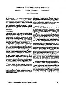
Figure 1a: Case studies
200 100 80
runtime (secs)
Source file LHashSet Stack HashSet TreeSet LHashMap ArrayList Vector PQueue LinkedList EnumMap Hashtable HashMap WHashMap IHashMap TreeMap Properties
coverage (%)
SLOC 9 17 46 62 103 150 200 203 227 239 355 360 384 392 562 2492
60 40 20 0
150
100
50
0 10
100
1000
SLOC
10
100
1000
SLOC
Figure 1b: SLOC vs line coverage. Median line coverage= 93%. Worst line coverage=3% from EnumMap.
Figure 1c: SLOC vs runtimes. Median runtimes ≈ 102 seconds. Larger cases studies do not necessarily have longer runtimes.
Figure 1: Nighthawk results from [1]. • Each call may be preceded by code that sets up the arguments and may be followed by code that stores and checks results.
Randomized unit testing uses coverage models that contain a bias on the random variables which select for the target method call sequence and/or arguments to the method calls. Many researchers [2, 6, 10, 21] have built such randomized coverage models, sometimes combined with other tools such as model checkers. However, these coverage models can also be learned. Previously [1], we have developed Nighthawk, a genetic algorithm (GA) for learning randomized coverage models. Nighthawk is a “wrapper” system that automates the construction of test scripts. Wrapper-based unit test generators are simpler to implement than (say) test generators that use model checkers [22] or static code analysis since these require access to a robust and complex parser and source code analyzers. These complex tools are not often provided by language providers and, if they are, they may not be updated to reflect recent changes in the source language. Nighthawk, on the other hand, does not require source code or bytecode analysis, instead depending only on the robust Java reflection mechanism and commonlyavailable coverage tools. For instance, our code was initially written with Java 1.4 in mind, but worked seamlessly on the Java 1.5 versions of the java.util classes, despite the fact that the source code of many of the units had been heavily modified to introduce templates. Nighthawk meets, and surpasses, the Cornett threshold [8]; i.e. “code coverage of 70-80% is a reasonable goal for system test of most projects with most coverage metrics”. Using a novel valuepool approach to coverage models, and running over the Java classes of Figure 1a, Nighthawk: • Achieves median coverage of 93% (measured in line coverage, see Figure 1b). • Achieves much higher coverage than other GA methods that ignore value pools [19] (measured in terms of condition/decision coverage); • Achieves similar coverage to other test coverage generators that use symbolic execution [1].
Hence, we prefer Nighthawk’s wrappers to symbolic methods since wrappers can be adapted to new languages faster than symbolic execution methods. Even though Nighthawk is a successful tool, it is still too slow to handle large code bases developed in an agile manner. As shown in Figure 1c, Nighthawk’s runtimes are usually in the order to 102 seconds per class. The goal of our current work is to speed up Nighthawk by two orders of magnitude3 . The rest of this paper discusses experiments with feature subset selection (FSS) and genetic algorithms (GAs). We will show that the RELIEF feature subset selector [16] consistently rejects 60% of our mutator operators over all the cases studies of Figure 1a. This results in a much larger speedup than 60% since the search space of a genetic algorithm is exponential on the number of mutators. Empirically we find that when we just use the mutators selected by RELIEF, we can usually (in 12 cases of 16) reach 94% of the coverage seen with all mutators, ten times as quickly. The Future Work section of this paper proposes an incremental feature subset selection method that might win us another order of magnitude speed improvement (but this has yet to be tested). That is, we can report good progress in our goal to achieving a speed up of 102 . The rest of this paper is structured as followed. Section 2 discusses related work. Section 3 describes the Nighthawk test input generation system. Section 4 describes how we applied feature subset selection (FSS) to data collected from Nighthawk in order to determine how best to optimize it. Section 5 explores future work; Section 6 concludes. Note one digression before continuing. To enhance availability of the software, Nighthawk uses the popular open-source coverage tool Cobertura [7] to measure coverage. Cobertura can measure only line coverage (each coverage point corresponds to a source
3
Of course, even faster would be even better but given our current case study library (Figure 1a), any speed up beyond 102 would become hard to detect. Before exploring 103 speedups, we would need to switch to much larger case studies.
code line, and is covered if any code on the line is executed)4 . However, Nighthawk’s algorithm is not specific to this measure; indeed, our other empirical studies [1] show that Nighthawk performs well when using other coverage measures.
2.
RELATED WORK
This paper focuses on optimizations of genetic algorithms building test coverage models for randomized unit testing. While the specifics of our techniques may not apply to other research, we suspect that the general problem explored here is relevant to other data mining research. This will be especially so for researchers exploring complex tasks in environments demanding greater speed. Some learning methods require very complex and costly computations which need to be reiterated every time the data changes. Many researchers use SVD (single value decomposition) for performing tasks related to program comprehension; for example, Marcus and Maletic [17] use it to find traceability links between documentation and source code based on terms. Once computed, the SVD results can be queried in millisecond time to find (say) the 10 methods closest to a particular method. This computation must be repeated whenever the code base changes; but in common practice, code base changes are becoming increasingly frequent. In order for the representation of the software system to be accurate, and for the tools to be able to help developers in real time during their daily activities, the current techniques would need to perform these complex computations over and over again, at an impractical computational cost. The complexity of SVD (single value decomposition) on a T ∗ D term*document matrix is O(min(T 2 D, T D2 )). In terms of algorithmic theory, this seems acceptable (since it is still polynomial time), but Marcus (personal communication) reports that, in practice, applying SVD over the large sparse T ∗ D matrices seen with real world code bases can take hours to days to compute.
Probability of covering 1 0.8 0.6 0.4 0.2 0
20 18 16 14 0
12 2
10 4
8
6
8
10
y
6 12
14
x
4 16
2 18
0
Figure 2: Spiky search space: the region x = y is very narrow.
Probability of covering 1 0.8 0.6 0.4 0.2 0
20 18 16 14
Many local learning schemes have slow runtimes. For example, Frank et al.’s [11] locally weighted Bayes classifier performs better than standard Bayes, but runs much more slowly since the neighborhood of each test case is computed at test time. In the worst case (when the test set is the entire training set, of size D) this search takes time O(D2 ) , since the distance between each pair of examples must be computed. While theoretically tractable, D2 can be impractically large. One way to optimize locally weighted learning schemes is to precompute and cache clusters that divide the space into pre-defined “chunks”. Each chunk is spatially indexed (e.g. using cover trees [4] or kd-trees [3]) so that local learning can be constrained to just their most relevant “chunk”. Note that this approach requires the recomputation of the clusters every time the training data changes. The techniques discussed in this paper do not necessarily solve the problems noted above. However, these problems show that the general research area of this paper is a looming problem for many SE data mining tasks. We therefore expect an increasing number of papers tackling the same theme of this paper (orders of magnitude runtime optimizations in learning method).
0
12 2
10 4
8
6
8
10
lo
6 12
hi
14
4 16
2 18
0
Figure 3: Smooth search space resulting from value pools.
Without value pools ------------------a = f1(); b = f2(); c = f3(); x = f4(a); y = f5(b); z = f6(c);
With value pools ---------------a = f1(); x = f4(a); y = f5(x); z = f6(y);
Figure 4: Unit tests without value pools (left) and with value pools (right). 4 Cobertura (v. 1.8) also reports what it calls “decision coverage”, but this is coverage of lines containing decisions.
3.
NIGHTHAWK
This section describes how the results in Figure 1 were generated using Nighthawk. We first discuss the notion of “value pool”, which Nighthawk uses to maintain candidate data for test cases. We then describe the genetic algorithm (GA) used by Nighthawk, and finally the algorithm used to randomly generate test data, which is based on the model discovered by the GA.
3.1
Value Pools
The core innovation in Nighthawk is that of value pools. A value pool is a collection of values of a given class shared between methods in a unit test; each relevant class corresponds to one or more value pools. Receivers and parameters of method calls are chosen from the appropriate value pool and possibly modified by the method call, and return values are deposited back in the value pool, to be possibly used as parameters or receivers in future method calls. The sharing of values has an interesting effect on the viability of randomized unit test generators like Nighthawk. To understand this effect, consider the problem of generating two input values x and y that will cover the true direction of the decision “x = y”. If we cast the problem as a search for the two values themselves, and the score as whether we have found two equal values, the search space is shaped as in Figure 2: a flat plain of zero score with spikes along the diagonal. Most approaches to GA white-box test data generation attempt to address this problem by proposing fitness functions that detect “how close” the target decision is to being true, often using analysis-based techniques. For instance, Michael et al. [19] use fitness functions that specifically take account of such conditions by measuring how close x and y are. Watkins and Hufnagel [23] enumerate and compare fitness functions proposed for GA-based test case generation. Now consider a random search for values satisfying x = y when x and y are calculated using value pools, where each value pool contains all the values between lo and hi. The reuse of values for a shared pool increases the probability of a choosing the same value for x and y, resulting in a search space more like Figure 3. We can generalize this to method calls in general. Without value pools, every value on the unit test on the left-hand side of Figure 4 comes from a different source. With value pools, we create fewer and share more variables. In the right-hand side revision of the unit test of Figure 4, the arguments to each function have a higher probability of coming from the results of prior function calls. Note that now there is a dependency between x and z (via y). Our search space is therefore more like Figure 3 and there is an increasing chance that random search will stumble on the sequence of calls that will achieve high coverage of the methods under test.
3.2
Genetic Algorithm
Nighthawk is given a set M of target methods, and finds values for genes that control randomized test data creation. We define the set IM of types of interest corresponding to M as the union of the following sets of types5 : • All types of receivers, parameters and return values of methods in M . • All primitive types that are the types of parameters to constructors of other types of interest. 5 In this paper, the word “type” refers to any primitive type, interface, or abstract or concrete class.
Each type t ∈ IM is associated with an array of value pools, and each value pool for t contains an array of values of type t. Each value pool for a range primitive type (a primitive type other than boolean and void) has bounds on the values that can appear in it. The number of value pools, number of values in each value pool, and the range primitive type bounds are specified by genes. We define a constructor to be a reinitializer if it has no parameters, or if all its parameters are of types in IM . We define the set CM of callable methods to be the methods in M plus the reinitializers of the types in IM . The callable methods are the ones that Nighthawk calls directly. Nighthawk’s genetic algorithm finds values for genes of various types; each gene type corresponds to zero or more genes of that type. One type of gene represents n (the number of method calls in this unit test) while another type selects the number of value pools for each datatype in IM . Yet another gene type selects the size of value pool for each datatype. The number of genes of each type thus varies according to the properties of the software unit under test. For example, Figure 5 shows that the methodWeight gene type is repeated for each method in M . The vector of all genes and their values is the chromosome used by Nighthawk. Our GA operates on this chromosome via the usual steps of chromosome evaluation, fitness selection, mutation and recombination. The GA first derives an initial template chromosome appropriate to M , constructs an initial population of size p as clones of this chromosome, and mutates the population. It then performs a loop, for the desired number g of generations, of evaluating each chromosome’s fitness, retaining the fittest chromosomes, discarding the rest, cloning the fit chromosomes, and mutating the genes of the clones with probability m% using point mutations and crossover (exchange of genes between chromosomes). The fitness function for a chromosome is calculated using the Cobertura coverage tool (discussed in the introduction): generally, chromosomes that cause the generation of test cases that achieve higher coverage are evaluated as being more fit. Nighthawk uses default settings of p = 20, g = 50, m = 20. These settings are different from those taken as standard in GA literature [9], and are motivated by a need to do as few chromosome evaluations as possible (the primary cost driver of the system). The settings of other variables, such as the retention percentage, are consistent with the literature.
3.3
Nighthawk
Here we present a simplified description of Nighthawk’s coveragemodel-based test case generation. The algorithm takes two parameters: a set M of Java methods, and a GA chromosome c appropriate to M . The chromosome controls aspects of the algorithm’s behaviour, such as the number of method calls to be made, as described in the previous subsection. The algorithm first chooses initial values for primitive type pools, and then moves on to non-primitive type pools. A call description is an object representing one method call that has been constructed and run. It consists of the method name, an indication of whether the method call succeeded, failed or threw an exception, and one object description for each of the receiver, the parameters and the result (if any). A test case is a sequence of call descriptions, together with an indication of whether the test case succeeded or failed.
Gene type numberOfCalls methodWeight
Occurrence One for whole chromosome One for each method m ∈ IM
numberOfValuePools numberOfValues
One for each type t ∈ CM One for each value pool of each type t ∈ CM except for boolean One for each value pool of type boolean
chanceOfTrue lowerBound, upperBound chanceOfNull candidateBitSet valuePoolActivityBitSet
Type int int
One for each value pool of each range primitive type t ∈ CM One for each argument position of non-primitive type of each method m ∈ IM One for each parameter and quasi-parameter of each method m ∈ IM One for each candidate type of each parameter and quasi-parameter of each method m ∈ IM
int int int int or float int BitSet BitSet
Description the number n of method calls to be made The relative weight of the method, i.e. the likelihood that it will be chosen The number of value pools for that type The number of values in the pool The percentage chance that the value true will be chosen from the value pool The lower and upper bounds on values in the pool; initial values are drawn uniformly from this range The percentage chance that null will be chosen as the argument Each bit represents one candidate type, and signifies whether the argument will be of that type Each bit represents one value pool, and signifies whether the argument will be drawn from that value pool
Figure 5: Nighthawk gene types. Input: a set M of target methods; a chromosome c. Output: a test case. Steps: 1. For each element of each value pool of each primitive type in IM , choose an initial value that is within the bounds for that value pool. 2. For each element of each value pool of each other type t in IM : (a) If t has no initializers, then set the element to null. (b) Otherwise, choose an initializer method i of t, call tryRunMethod(i, c), and place the result in the destination element. 3. Initialize test case k to the empty test case. 4. Repeat n times, where n is the number of method calls to perform: (a) Choose a target method m ∈ CM . (b) Run algorithm tryRunMethod(m, c), and add the call description returned to k. (c) If tryRunMethod returns a method call failure indication, return k with a failure indication. 5. Return k with a success indication.
Input: a method m; a chromosome c. Output: a call description. Steps: 1. If m is non-static and not a constructor: (a) Choose a type t ∈ IM which is a subtype of the receiver of m. (b) Choose a value pool p for t. (c) Choose one value recv from p to act as a receiver for the method call. 2. For each argument position to m:
Figure 6: Algorithm constructRunTestCase. Nighthawk’s randomized testing algorithm is referred to as constructRunTestCase, and is described in Figure 6. It takes a set M of target methods and a chromosome c as inputs. It begins by initializing value pools, and then constructs and runs a test case, and returns the test case. It uses an auxiliary method called tryRunMethod, described in Figure 7, which takes a method as input, calls the method and returns a call description. In the algorithm descriptions, the word “choose” is always used to mean specifically a random choice which may partly depend on the chromosome c. tryRunMethod considers a method call to fail if and only if it throws an AssertionError. It does not consider other exceptions to be failures, since they might be correct responses to bad input parameters. A separate mechanism is used for detecting precondition violations and checking correctness of return values and exceptions.
3.4
Generation of Results
We ran Nighthawk on each of the subject units in Figure 1a, all taken from the standard java.util library, version 1.5. The amount of coverage achieved by the “winning” chromosome on the units is graphed against unit SLOC in Figure 1b, and the amount of time taken to achieve highest coverage is graphed against unit
(a) Choose a type t ∈ IM which is a subtype of the argument type. (b) Choose a value pool p for t. (c) Choose one value v from p to act as the argument. 3. If the method is a constructor or is static, call it with the chosen arguments. Otherwise, call it on recv with the chosen arguments. 4. If the method call threw an AssertionError, return a call description with a failure indication. 5. Otherwise, if the method call threw some other exception, return a call description with an exception indication. 6. Otherwise, if the method return type is not void, and the return value ret is non-null: (a) Choose a type t ∈ IM which is a supertype of the type of the return value. (b) Choose a value pool p for t. (c) If t is not a primitive type, or if t is a primitive type and ret does not violate the bounds on p, then choose an element of p and replace it by ret. (d) Return a call description with a success indication.
Figure 7: Algorithm tryRunMethod.
SLOC in Figure 1c. Note that there is no particular pattern in the runtimes. For more details, see Andrews et al. [1].
WRAPPER where 83% (on average) of the measures in a domain could be ignored with only a minimal loss of accuracy.
This concludes our notes on how Figure 1 was generated. The rest of this paper concerns how to optimize the above process.
The advantage of the WRAPPER approach is that, if some target learner is already implemented, then the WRAPPER is simple to implement. The disadvantage of the wrapper method is that each step in the heuristic search requires another call to the target learner. Since there are many steps in such a search (N features have 2N subsets), WRAPPERs may be too slow.
4.
FEATURE SUBSET SELECTION
Here we describe the work that we have done to optimize Nighthawk’s GA and test case generation using feature subset selection (FSS). We first give some motivation, and then describe the data collection and initial FSS analysis of Nighthawk. We then describe the efficiency study that we carried out based on the information from FSS, with respect to both coverage and time.
4.1
Motivation
The size of the search space of a GA is the product of all possible values for all parts of a chromosome. The run time cost to find the best possible chromosome is therefore proportional to this value times the evaluation cost of each chromosome: cost = RL ∗ eval
(1)
That is, a chromosome of length L = 20 with binary choices (so the range of each choice is R = 2) takes 210 > 1, 000 times longer to run than a chromosome of length 10 to achieve the same quality of result. Nighthawk’s chromosomes store information related to the gene types of Figure 5. If we could discard some of those gene types, then the above reasoning suggests that this would lead to an exponential improvement in Nighthawk’s runtimes. One tool for removing needless information is feature subset selection (FSS). A repeated result in the data mining community is that simpler models with equivalent or higher performance can be built via FSS, algorithms that intelligently prune useless features [12]. Features may be pruned for several reasons: • They may be noisy, i.e. contain spurious signals unrelated to the target class; • They may be uninformative, e.g. contain mostly one value, or no repeating values; • They may be correlated to other variables; i.e. they can be pruned since their signal is also present in other variables. The reduced feature set has many advantages: • Miller has shown that models generally containing fewer variables have less variance in their outputs [20]. • The smaller the model, the fewer are the demands on interfaces (sensors and actuators) to the external environment. Hence, systems designed around small models are easier to use (less to do) and cheaper to build. • As argued above, for GAs a linear decrease in the number of chromosomes could lead to an exponential decrease in runtimes. The literature lists many feature subset selectors. In the WRAPPER method, a target learner is augmented with a pre-processor that uses a heuristic search to grow subsets of the available features. At each step in the growth, the target learner is called to find the accuracy of the model learned from the current subset. Subset growth is stopped when the addition of new features does not improve the accuracy. Kohavi and John [14] report experiments with
Another feature subset selector is RELIEF. This is an instance based learning scheme [13, 15] that works by randomly sampling one instance within the data. It then locates the nearest neighbors for that instance from not only the same class but the opposite class as well. The values of the nearest neighbor features are then compared to that of the sampled instance and the feature scores are maintained and updated based on this. This process is specified for some userspecified number M of instances. RELIEF can handle noisy data and other data anomalies by averaging the values for K nearest neighbors of the same and opposite class for each instance [15]. For data sets with multiple classes, the nearest neighbors for each class that is different from that of the current sampled instance are selected and the contributions are determined by using the class probabilities of the class in the dataset. The experiments of Hall and Holmes [12] reject numerous feature subset selection methods. WRAPPER is their preferred option, but only for small data sets. For larger data sets, the stochastic nature of RELIEF makes it a natural choice.
4.2
Initial FSS Analysis of Nighthawk
We instrumented Nighthawk so that every time a chromosome was evaluated, it printed the current value of every gene and the final fitness function score. (For the two BitSet gene types, we printed only the cardinality of the set.) For each of the 16 Collection and Map classes from java.util, we ran Nighthawk for 40 generations. Each class therefore yielded 800 observations, each consisting of a gene value vector and the chromosome score. RELIEF assumes discrete data and Nighthawk’s performance scores are continuous. To enable feature subset selection, we first discretized Nighthawk’s output. A repeated pattern across all our experiments is that the Nighthawk scores fall into three regions: • The 65% majority of the scores are within 30% of the top score for any experiment. We call this the high plateau. • A 10% minority of scores are less than 10% of the maximum score. We call this region the hole. • After the high plateau there is a slope of increasing gradient that falls into the hole. This slope accounds for 25% of the results. Accordingly, to select our features, we sorted the results and divided them into three classes: bottom 10%, next 25%, remaining 65%. RELIEF then found the subset of features that distinguished these three regions. Using the above discretization policy, we ran RELIEF 10 times in a 10-way cross-validation study. The data set was divided into 10 buckets. Each bucket was (temporarily) removed and RELIEF was run on the remaining data. This produced a list of “merit” figures for each feature (this “merit” value is an internal heuristic measure generated from RELIEF, and reflects the difference ratio of neigh-
Gene type t candidateBitSet upperBound valuePoolActivityBitSet numberOfCalls numberOfValuePools chanceOfNull numberOfValues chanceOfTrue methodWeight lowerBound
bestM erit(t) 0.373 0.267 0.267 0.195 0.186 0.166 0.160 0.150 0.144 0.129
Figure 8: Nighthawk gene types, sorted by the maximum RELIEF merit of any of its features. boring instances that have different regions). We therefore got a merit score for each of the ten runs for every gene corresponding to every subject unit. Each run therefore yielded a ranked list R of all genes, where gene 1 had the highest merit for this run, gene 2 had the second highest merit, and so on.
1.05 1 % max coverage
Rank 1 2 3 4 5 6 7 8 9 10
1 2 3 4 5 6 7 8 9 10
0.95 0.9 0.85 0.8 0.75 0
We then calculated various summary statistics in order to come up with rankings of the various gene types (recall that each gene type t corresponds to zero or more genes, depending on the unit under test). • avgM erit(g, u) is the average RELIEF merit score, across all 10 runs of the cross-validation study, of gene g derived from unit u.
10
20
30 40 50 generations
60
70
Figure 9: Nighthawk on Hashtable unit, eliminating gene types according to bestM erit ranking.
• avgRank(g, u) is the average rank in R, across all 10 runs of the cross-validation study, of gene g derived from unit u. • bestM erit(t) is the maximum, over all genes g of type t and all subject units u, of avgM erit(g, u). • bestRank(t) is the maximum, over all genes g of type t and all subject units u, of avgRank(g, u).
4.3
Efficiency Study
After ranking the gene types by the various ranking metrics, we proceeded to study whether eliminating gene types on the basis of the RELIEF results sped up Nighthawk without sacrificing the quality of the results.
1.05
% max coverage
We took these summary numbers as indications of the possible relative expendibility of the various different gene types. For example, Figure 8 shows the ten gene types from Figure 5, ranked in terms of their best merit as defined above. This ranking places candidateBitSet at the top, meaning that it considers genes of that type to be the most valuable; it also places lowerBound at the bottom, meaning that it considers genes of that type to be the most expendible.
1 1 2 3 4 5 6 7 8 9 10
0.95 0.9 0.85 0.8 0
First, we instrumented the source code so that we could selectively replace the parts of Nighthawk’s code controlled by each gene type by code that assumed a constant value for each gene of that type. This allowed us to “turn off” all genes of a given type. We then ran Nighthawk using the top ranked 1 ≤ i ≤ 10 gene types according to two rankings: the ranking by bestM erit shown in Figure 8, and the ranking by bestRank. For example, in the following experiments, if we say “number of gene types = 2” for the bestM erit ranking, then we are using only candidateBitSet and upperBound, and all other gene types are turned off.
10
20
30 40 50 generations
60
70
Figure 10: Nighthawk on Hashtable unit, eliminating gene types according to bestRank ranking.
Number of used gene types 1 2 3 4 5 6 7 8 9 10 .91 .92 .92 1.00 1.01 1.01 1.01 1.01 1.00 1.00 .89 .89 .90 1.01 1.01 1.00 .99 1.01 1.01 1.00 1.21 1.11 1.19 1.20 1.21 1.57 1.13 1.32 1.29 1.00 .83 .86 .85 .98 .99 1.00 1.00 1.00 .98 1.00 .92 .91 .92 1.01 .99 1.00 1.01 1.00 .99 1.00 .86 .88 .89 1.01 1.00 1.01 1.02 . 99 .99 1.00 .84 .86 .84 1.02 1.01 1.01 1.01 1.00 1.02 1.00 .93 .93 .94 1.01 1.01 1.01 1.01 1.01 1.01 1.00 .93 .92 .92 1.01 1.00 1.01 1.00 1.00 1.01 1.00 .87 .87 .88 1.02 1.00 1.01 1.02 1.05 1.05 1.00 .99 .97 .99 1.00 1.00 1.01 1.00 1.00 1.00 1.00 .94 .93 .93 1.01 1.01 1.01 1.00 1.01 1.01 1.00 .75 .78 .77 .98 .98 .99 0.90 1.00 .98 1.00 .82 .81 .82 1.01 .99 1.03 1.02 1.01 1.00 1.00 .77 .82 .77 1.01 1.00 1.04 1.02 1.03 1.01 1.00 .87 .89 .87 1.01 1.00 1.03 1.00 .99 1.01 1.00 .90 .90 .90 1.02 1.01 1.05 1.01 1.03 1.02 1.00
class being tested Hashtable ArrayList EnumMap HashMap HashSet IdentityHashMap LinkedHashMap LinkedHashSet LinkedList PriorityQueue Properties Stack TreeMap TreeSet Vector WeakHashMap mean
Figure 11: Coverage found using the top 1i ranked gene types for 0 ≤ i ≤ 9 Coverages expressed as a ratio of the coverages found using all gene types
4.3.1
other rankings of genes, in an attempt to find a ranking that best identifies the most useful gene types.
4.3.2
Time Analysis
In order to determine whether eliminating gene types from Nighthawk’s GA is cost-effective, we must consider not only the coverage achievable, but also the time taken to achieve that coverage. We therefore made two runs of Nighthawk on all the subject units, run (a) using all the gene types and run (b) using just the top four gene types ranked by bestM erit. We then divided the runtime and coverage results from (b) by the (a) values seen after 50 generations, and plotted the results. Figure 12 shows the results, with time percentage on the X axis and coverage percentage on the Y axis. For example, the graph shows that in the Vector results, using four gene types achieved 100% of the coverage found using all types, but took approximately 100% longer to do so. Note the point indicated by the arrow in Figure 12. cases) possible to achieve This point shows that it is usually (in 12 16 94% of the coverage in under 10% of the time required to run all gene types for 50 generations.
Coverage Analysis
In the following, the result of each run is always compared to the runtime and coverage seen using all ten gene types and running for g = 50 generations. Figure 9 shows how the coverage changed over one of the case studies of Figure 1, using the bestM erit ranking; the results for this subject unit are typical. The y-axis of that figure is defined such that the point (50,1) represents the coverage reached by using all 10 gene types after 50 generations. The thick black curve on those figures shows the performance of Nighthawk using all ten gene types. The other curves show results from using 1 ≤ i ≤ 9 gene types. The corresponding plot for the bestRank ranking is shown in Figure 10. A performance measure of interest in Figure 9 is the area under the curves. This area is maximal when Nighthawk converges to maximum coverage in only a few generations. Note that due to the random nature of the GA and the randomized test data generation, some of the curves are sometimes higher than the i = 10 line. If we calculate the ratio of the area under a curve with the area under the thick black curve, then we can summarize all the curves of Figure 9 as the first row of Figure 11. In that figure, each column shows how many gene types were used in a particular run (and when used = 10, we are ignoring the FSS results and using all gene types). Also, the number 1.00 informs us that we achieved 100% of the coverage reached by using all ten gene types. Figure 11 summarizes Figure 9 as well as results from all other cases studied in Figure 1a. The coverage is less than one for columns (1,2,3) but predominantly equal to or greater than one for columns (4-10). From this observation, we conclude that Nighthawk’s GA need only use the top four ranked gene types of Figure 8. The results for the bestRank ranking are less useful, as suggested by Figure 10: by that ranking, the top six gene types are needed for performance that comes close to all ten gene types. We note that in both the study using the bestM erit ranking and that using the bestRank ranking, the coverage achieved after 50 generations dropped off significantly at the point that we turned off the numberOfCalls gene. This suggests that the numberOfCalls gene may be more important than is suggested by either the bestM erit ranking or the bestRank ranking. We plan in the future to consider
The two anomalous subject units in Figure 12 are EnumMap and Vector. EnumMap looks like a success story, since we were able to achieve 140% of the original coverage. In fact, this is simply noise, since we could achieve only 3% coverage of EnumMap using Nighthawk and generic test wrappers [1], and the graph shows an improvement to less than 5%. To understand the Vector results, note that Equation 1 has two components: number of options and the evaluation cost of each option. In the case of Vector, even though we reduced the chromosome search space size, we made choices that greatly increased the runtime cost. What do all these numbers mean to the Nighthawk system? In a nutshell, they mean that the original Nighthawk was doing much work that did not pay off by achieving much better results. Consider the six gene types ranked the lowest in the bestM erit ranking. Maintaining all the genes associated with these gene types meant that the original Nighthawk was spending time mutating these genes and extracting information from the current values of the genes; it also meant that the original Nighthawk was using up memory storing the representations of these genes, for each chromosome in each generation, with a concomitant time expense. When these less useful genes were eliminated, no large loss of coverage was observed, but a great increase in efficiency was observed.
5.
IMPLICATIONS FOR FUTURE WORK
We see implications of this work on three levels, each of which we would like to explore: on the tool level, the metaheuristic level, and the theory-formation level. On the tool level, this work shows that it is viable to use feature subset selection as a postprocessing step in order to improve the performance of a metaheuristic tool. Metaheuristic tools (such as genetic algorithms and simulated annealers) typically mutate some aspect of a candidate solution and evaluate the results. If the effect of mutating each aspect is recorded, then each aspect can be considered a feature and is amenable to the FSS processing described here. Another impact on the tool level is to suggest stopping criteria for metaheuristic algorithms; for instance, Figure 12 suggests that for Nighthawk’s GA, ending the algorithm when a time limit is reached
140 130
% max coverage (4 types)/(10 types)
120
EnumMap
Vector
110 100 ArrayList EnumMap HashMap HashSet HashTable IdentityHashMap LinkedHashMap LinkedHashSet LinkedList PriorityQueue Properties Stack TreeMap TreeSet Vector WeahHashMap
90 80
time= 10%, coverage= 94%
70 60 50 40 0
50
100
150
200
250
% time using (4 types)/(10 types)
Figure 12: Time results, 4 vs 10. or when the fitness function has remained constant for several generations will usually result in a good cost-effectiveness tradeoff. In this work, we have not directly considered time as a cost factor in the FSS analysis, but we could do so by directly calculating the cost-effectiveness of the gene types and removing first the ones that are least cost-effective. A final impact on the tool level is to facilitate the introduction and evaluation of other gene types. In constructing a genetic algorithm for a tool, the tool designer makes choices of what aspects to control by genes and what aspects to hard-code. It is possible that we simply made poor initial choices when deciding which aspects to control by genes (although Figures 9 and 10 suggest that most genes have at least some impact on coverage). The availability of FSS analysis allows us to easily experiment with controlling more or different aspects of the algorithm with genes, winnowing out those genes that do not yield a good return on time investment. On the metaheuristic level, this work suggests that it may be useful to integrate FSS directly into metaheuristic algorithms. Such an integration would enable the automatic reporting of the merits of individual features, and the automatic or semi-automatic selection of features. If the results of this paper extend to other domains, this would lead to metaheuristic algorithms that improve themselves automatically each time they are run. We also speculate that this is a promising direction to look at for a further order of magnitude improvement in performance. Finally, on the theory-formation level, this work opens up the possibility of rapid turnover of the theoretical foundations underlying present tools, as aspects of heuristic and meta-heuristic approaches are shown to be consistently valuable or expendible. In the framework of a self-monitoring metaheuristic algorithm, new strategies, heuristics, and gene and mutator types can be introduced as theories
evolve, and can be evaluated efficiently by the algorithms themselves. As an example of this latter point, the chanceOfNull gene type in Nighthawk determines how likely (in percent) Nighthawk’s random test data generation is to choose a null as a parameter in a given parameter position. That gene type was ranked as expendible by both rankings explored here. This suggests that it is not worthwhile to search for different values for this percentage, and that the default value (3%) is sufficient. Given sufficient corroboration from other case studies and systems, this in turn suggests that the value of generating test data with nulls is a relatively settled problem, and that we can turn toward other aspects of test data generation for future improvements.
6.
CONCLUSION
We applied feature subset selection (FSS) to a metaheuristic algorithm used to learn coverage models for randomized unit test generation. FSS allowed us to cut down on the number of gene types we used, without a noticeable loss of coverage. Since each gene type corresponded to runtime cost, this also allowed us to cut down on the time and memory taken for the algorithm. These are preliminary results only, but are suggestive. In the future, we wish to study the use of FSS to speed up other heuristic and metaheuristic software engineering tools. We also wish to explore the impact of FSS on all three of the levels noted above (tool, metaheuristic, and theory-formation).
Acknowledgment Thanks for interesting comments and discussions to Rob Hierons, Charles Ling, Bob Mercer and Andy Podgurski. This research is supported by the first author’s grant from the Natural Sciences and Research Council of Canada (NSERC).
7.
REFERENCES
[1] J. Andrews, F. Li, and T. Menzies. Nighthawk: A two-level genetic-random unit test data generator. In IEEE ASE’07, 2007. Available from http: //menzies.us/pdf/07ase-nighthawk.pdf. [2] S. Antoy and R. G. Hamlet. Automatically checking an implementation against its formal specification. IEEE Transactions on Software Engineering, 26(1):55–69, January 2000. [3] J. Bentley. K-d trees for semidynamic point sets. In Proceedings Proceedings of the 6th Annual Symposium on Computational Geometry, Berkley, California, United States, pages 187–197, 1990. [4] A. Beygelzimer, S. Kakade, and J. Langford. Cover trees for nearest neighbor. In ICML’06, 2006. Available from http://hunch.net/˜jl/projects/cover_ tree/cover_tree.html. [5] F. Brooks. No silver bullet: Essence and accidents of software engineering. IEEE Computer, 20(4):34–42, 1987. [6] K. Claessen and J. Hughes. QuickCheck: A lightweight tool for random testing of Haskell programs. In Proceedings of the Fifth ACM SIGPLAN International Conference on Functional Programming (ICFP ’00), pages 268–279, Montreal, Canada, September 2000. [7] Cobertura Development Team. Cobertura web site. cobertura.sourceforge.net, accessed February 2007. [8] S. Cornett. Minimum acceptable code coverage. http://www.bullseye.com/minimum.html, 2006. [9] K. A. DeJong and W. M. Spears. An analysis of the interacting roles of population size and crossover in genetic algorithms. In First Workshop on Parallel Problem Solving from Nature, pages 38–47. Springer, 1990. [10] R.-K. Doong and P. G. Frankl. The ASTOOT approach to testing object-oriented programs. ACM Transactions on Software Engineering and Methodology, 3(2):101–130, April 1994. [11] E. Frank, M. Hall, and B. Pfahringer. Locally weighted naive bayes. In Proceedings of the Conference on Uncertainty in Artificial Intelligence, pages 249–256. Morgan Kaufmann, 2003. [12] M. Hall and G. Holmes. Benchmarking attribute selection techniques for discrete class data mining. IEEE Transactions On Knowledge And Data Engineering, 15(6):1437– 1447, 2003. [13] K. Kira and L. Rendell. A practical approach to feature selection. In The Ninth International Conference on Machine Learning, pages pp. 249–256. Morgan Kaufmann, 1992. [14] R. Kohavi and G. H. John. Wrappers for feature subset selection. Artificial Intelligence, 97(1-2):273–324, 1997. [15] I. Kononenko. Estimating attributes: Analysis and extensions of relief. In The Seventh European Conference on Machine Learning, pages pp. 171–182. Springer-Verlag, 1994. [16] I. Kononenko, E. Simec, and M. Robnik-Sikonja. Overcoming the myopia of inductive learning algorithms with relieff. Applied Intelligence, 7:39–55, 1997. Available from http://citeseerx.ist.psu.edu/viewdoc/ summary?doi=10.1.1.56.4740. [17] A. Marcus and J. Maletic. Recovering documentation-to-source code traceability links using latent semantic indexing. In Proceedings of the Twenty-Fifth
International Conference on Software Engineering, 2003. [18] T. Menzies, J. Greenwald, and A. Frank. Data mining static code attributes to learn defect predictors. IEEE Transactions on Software Engineering, January 2007. Available from http://menzies.us/pdf/06learnPredict.pdf. [19] C. C. Michael, G. McGraw, and M. A. Schatz. Generating software test data by evolution. IEEE Transactions on Software Engineering, 27(12), December 2001. [20] A. Miller. Subset Selection in Regression (second edition). Chapman & Hall, 2002. [21] C. Pacheco, S. K. Lahiri, M. D. Ernst, and T. Ball. Feedback-directed random test generation. In Proceedings of the 29th International Conference on Software Engineering (ICSE 2007), pages 75–84, Minneapolis, MN, May 2007. [22] W. Visser, C. S. P˘as˘areanu, and R. Pel´anek. Test input generation for Java containers using state matching. In Proceedings of the International Symposium on Software Testing and Analysis (ISSTA 2006), pages 37–48, Portland, Maine, July 2006. [23] A. Watkins and E. M. Hufnagel. Evolutionary test data generation: A comparison of fitness functions. Software Practice and Experience, 36:95–116, January 2006.