Fault Tolerant Adaptive Routing in Multicomputer Networks - CiteSeerX

Fault Tolerant Adaptive Routing in Multicomputer Networks by

Thucydides Xanthopoulos

B.S.E.E., Massachusetts Institute of Technology (1992) Submitted to the Department of Electrical Engineering and Computer Science In Partial Ful llment of the Requirements for the Degree of Master of Science in Electrical Engineering and Computer Science at the Massachusetts Institute of Technology February 1995

c 1995 Thucydides Xanthopoulos. All rights reserved. The author hereby grants to MIT permission to reproduce and to distribute copies of this thesis document in whole or in part. Signature of Author Department of Electrical Engineering and Computer Science January 20, 1995 Certi ed by William J. Dally Associate Professor of Electrical Engineering and Computer Science Thesis Supervisor Accepted by Frederic R. Morgenthaler Chairman, Departmental Committee on Graduate Students

Fault Tolerant Adaptive Routing in Multicomputer Networks by

Thucydides Xanthopoulos

Submitted to the Department of Electrical Engineering and Computer Science on January 20, 1995, in partial ful llment of the requirements for the Degree of Master of Science in Electrical Engineering and Computer Science

Abstract Interconnection networks play a major role in the performance and reliability of massively parallel processors (MPPs). This work is concerned with the design and implementation of a wormhole fault-tolerant adaptive routing algorithm for k-ary n-meshes called Reliable Adaptive Routing (RAR). RAR when coupled with a fault-detection mechanism and a retransmission protocol is capable of handling a single link or node failure anywhere in the network without interruption of service. Furthermore, RAR can assign multiple message paths between each source and destination pair. RAR uses virtual channels to prevent deadlocks. A total of three virtual channels per physical channel are necessary for deadlock prevention. The routing algorithm is formally de ned and a formal proof of deadlock freedom is presented. This work also presents the Virtual Channel Dependency Analyzer (VCDA) a software tool with a graphical user interface that helps in the visualization and study of the channel dependency graph produced by Reliable Adaptive Routing. A sample circuit implementation of RAR is also presented. The circuit uses 236m  904m of silicon area and has a worst case delay of 6 ns. This work concludes by describing higher level design issues such as the integration of the above circuit in a complete routing system, and also the coupling with a retransmission protocol to produce a reliable network layer. Thesis Supervisor: William J. Dally Title: Associate Professor of Electrical Engineering and Computer Science

Keywords: Adaptive routing, virtual channels, channel dependency graph, reliable rout-

ing, fault tolerance.

4

Dedication ? o o! (1963 ? 1992)

M o&  o: T!  & oo :  !o  !      : E  Ko; !o&; o&; o&;  &;   o: E !  Bo!; oo&; o&; o o  oo   !&: E o oo   !  :  oo&   &   o: T& !   o& o& o  : !&  &   o: You were seven years older than me. Now, you are just four years older. In the picture above, we probably have the same age. You are in Kalymnos, handsome, strong, tanned, having fun, wearing sunglasses. I am in Boston, fat, pathetic, in front of a computer screen wearing prescription glasses. You are in heaven, I am still in earth. You look ready to tell a story again. I have believed them all except for one: That you will always be twenty-nine. 5

6

Acknowledgments I would like to thank a number of people that have contributed to one way or another to the completion of this project:

 Bill Dally for his energy, enthusiasm and most constructive supervision.  Larry Dennison for his valuable experience and enormous patience.  All the past and present members of the Reliable Router team including Larry Dennison, Kin Hong Kan, David Harris, Ivan Oei, Dan Hartman and Je Bowers for their valuable contributions to our project.

 All the members of the CVA group for providing a most pleasant and stimulating

work environment. I would like to thank especially Rich Lethin for volunteering to proofread the most basic chapters of this thesis.

 All my friends here in Boston, especially Sylvi Dogramatzian for helping me get a life!  Finally, I would like to thank my parents Maria and Nicholas Xanthopoulos as well as my uncle John Xanthopoulos for their invaluable love and support throughout all these years that I have been away.

7

8

Contents 1 Introduction

17

2 Background

21

1.1 A Case for Adaptive Routing : : : : : : : : : : : : : : : : : : : : : : : : : : 1.2 Contributions of this work : : : : : : : : : : : : : : : : : : : : : : : : : : : : 1.3 Thesis Overview : : : : : : : : : : : : : : : : : : : : : : : : : : : : : : : : :

2.1 2.2 2.3 2.4 2.5 2.6 2.7 2.8 2.9 2.10

Evaluation Criteria : : : : : : : : : : : : : : The Linder-Harden Algorithm : : : : : : : : Planar Adaptive Routing : : : : : : : : : : The Turn Model For Adaptive Routing : : Dimension Reversals : : : : : : : : : : : : : Compressionless Routing : : : : : : : : : : : Pipelined Circuit Switching : : : : : : : : : f-cube3 Algorithm : : : : : : : : : : : : : : Duato's New Theory on Adaptive Routing : Summary and Conclusion : : : : : : : : : :

: : : : : : : : : :

: : : : : : : : : :

: : : : : : : : : :

: : : : : : : : : :

: : : : : : : : : :

: : : : : : : : : :

: : : : : : : : : :

: : : : : : : : : :

: : : : : : : : : :

: : : : : : : : : :

: : : : : : : : : :

: : : : : : : : : :

: : : : : : : : : :

: : : : : : : : : :

: : : : : : : : : :

: : : : : : : : : :

: : : : : : : : : :

: : : : : : : : : :

3 De nitions, Theorems and Notation 3.1 Notation : : : : : : : : : : : : : : : : : : : : : : : : : : : : : : : : : : : : : : 3.2 De nitions : : : : : : : : : : : : : : : : : : : : : : : : : : : : : : : : : : : : : 3.3 Theorems : : : : : : : : : : : : : : : : : : : : : : : : : : : : : : : : : : : : : 9

17 19 20

21 22 23 24 26 26 27 28 30 30

32 32 32 35

4 Adaptive Routing

4.1 Informal Description : : : : : : : 4.2 Formal Description : : : : : : : : 4.2.1 Notation : : : : : : : : : : 4.2.2 De ning R and R1 : : : : 4.3 Facts about R and R1 : : : : : : 4.4 Proving Freedom from Deadlock 4.5 Summary : : : : : : : : : : : : :

: : : : : : :

: : : : : : :

5 Reliable Adaptive Routing

: : : : : : :

: : : : : : :

: : : : : : :

: : : : : : :

: : : : : : :

: : : : : : :

: : : : : : :

: : : : : : :

: : : : : : :

: : : : : : :

: : : : : : :

: : : : : : :

5.1 Fault Model : : : : : : : : : : : : : : : : : : : : : : : : : : 5.2 Informal Description : : : : : : : : : : : : : : : : : : : : : 5.2.1 Examples : : : : : : : : : : : : : : : : : : : : : : : 5.2.2 The Algorithm : : : : : : : : : : : : : : : : : : : : 5.3 Formal De nition : : : : : : : : : : : : : : : : : : : : : : : 5.3.1 Notation : : : : : : : : : : : : : : : : : : : : : : : : 5.3.2 De ning R and R2 : : : : : : : : : : : : : : : : : : 5.4 Facts About Reliable Adaptive Routing : : : : : : : : : : 5.4.1 Fault Along a Dimension d 6= 0 : : : : : : : : : : : 5.4.2 Fault Along Dimension 0 : : : : : : : : : : : : : : 5.5 Proof of Deadlock Freedom : : : : : : : : : : : : : : : : : 5.5.1 Fault along the x dimension : : : : : : : : : : : : : 5.5.2 Fault along the y dimension : : : : : : : : : : : : : 5.5.3 Proving Deadlock Freedom In Two Dimensions : : 5.6 Extending the Proof to Arbitrary Dimensions : : : : : : : 5.6.1 Fault Along Dimension n ? 1. : : : : : : : : : : : : 5.6.2 Fault Along Dimension d such that 0 < d < n ? 1 : 5.6.3 Fault Along Dimension 0 : : : : : : : : : : : : : : 5.6.4 Proving Deadock Freedom in n Dimensions : : : : 5.7 Summary : : : : : : : : : : : : : : : : : : : : : : : : : : : 10

: : : : : : : : : : : : : : : : : : : : : : : : : : :

: : : : : : : : : : : : : : : : : : : : : : : : : : :

: : : : : : : : : : : : : : : : : : : : : : : : : : :

: : : : : : : : : : : : : : : : : : : : : : : : : : :

: : : : : : : : : : : : : : : : : : : : : : : : : : :

: : : : : : : : : : : : : : : : : : : : : : : : : : :

: : : : : : : : : : : : : : : : : : : : : : : : : : :

: : : : : : : : : : : : : : : : : : : : : : : : : : :

: : : : : : : : : : : : : : : : : : : : : : : : : : :

: : : : : : : : : : : : : : : : : : : : : : : : : : :

37 37 40 40 40 43 46 48

49 49 50 50 51 53 53 53 57 58 58 59 61 68 68 70 70 70 70 70 71

6 The Virtual Channel Dependency Analyzer

72

6.1 Functional Description : : : : : : : : : : : : : 6.2 A Sample Session with VCDA : : : : : : : : : 6.2.1 Program Manager : : : : : : : : : : : 6.2.2 Building and Displaying the Network : 6.2.3 Creating the Dependency Graph : : : 6.2.4 Looking for Deadlocks : : : : : : : : : 6.2.5 Placing Faults : : : : : : : : 6.3 VCDA Internals : : : : : : : : : : : 6.3.1 Object Representation : : : : 6.3.2 The Cycle-Search Algorithm 6.3.3 Interfacing Tcl and C : : : : 6.4 Future Work : : : : : : : : : : : : : 6.5 Summary : : : : : : : : : : : : : : :

: : : : : : :

: : : : : : :

: : : : : : :

: : : : : : :

: : : : : : :

: : : : : : : : : : : : :

: : : : : : : : : : : : :

: : : : : : : : : : : : :

: : : : : : : : : : : : :

: : : : : : : : : : : : :

: : : : : : : : : : : : :

: : : : : : : : : : : : :

: : : : : : : : : : : : :

: : : : : : : : : : : : :

: : : : : : : : : : : : :

: : : : : : : : : : : : :

: : : : : : : : : : : : :

: : : : : : : : : : : : :

: : : : : : : : : : : : :

: : : : : : : : : : : : :

: : : : : : : : : : : : :

7 Implementation Issues

72 73 73 73 74 74 78 80 80 86 87 88 89

90

7.1 Input and Output Speci cation : : : : : : : : : : : : : : 7.1.1 Routing Problem : : : : : : : : : : : : : : : : : : 7.1.2 Output Virtual Channel Availability Information 7.1.3 Port Status Information : : : : : : : : : : : : : : 7.1.4 Routing Answer : : : : : : : : : : : : : : : : : : 7.2 Optimizing Circuit Latency : : : : : : : : : : : : : : : : 7.2.1 Parallel Computations : : : : : : : : : : : : : : : 7.3 7.4 7.5 7.6

: : : : : : : : : : : : :

: : : : : : : 7.2.2 Preprocessing Output Virtual Channel Availability Information : Logic Circuit Schematics : : : : : : : : : : : : : : : : : : : : : : : : : : : Logic Simulation and Validation : : : : : : : : : : : : : : : : : : : : : : Determining Circuit Delay : : : : : : : : : : : : : : : : : : : : : : : : : : Circuit Layout : : : : : : : : : : : : : : : : : : : : : : : : : : : : : : : : 11

: : : : : : :

: : : : : : :

: : : : : : :

: : : : : : :

: : : : : : :

: : : : : : :

: : : : : : :

: : : : : : :

: : : : : : : : : : : :

: 90 : 91 : 92 : 93 : 93 : 94 : 94 : 94 : 97 : 99 : 101 : 101

7.6.1 Determining Latency Using Extracted Layout : : : : : : : : : : : : : 104 7.7 Layout Veri cation : : : : : : : : : : : : : : : : : : : : : : : : : : : : : : : : 104 7.8 Summary : : : : : : : : : : : : : : : : : : : : : : : : : : : : : : : : : : : : : 105

8 The Big Picture

106

8.1 Brief Architectural Description : : : : : : : : : : : : : : : : : : : : : : : : : 106 8.2 The Unique Token Protocol : : : : : : : : : : : : : : : : : : : : : : : : : : : 109 8.2.1 Fault Handling : : : : : : : : : : : : : : : : : : : : : : : : : : : : : : 110 8.2.2 Flit-Level Implementation of the UTP : : : : : : : : : : : : : : : : : 111 8.3 Summary : : : : : : : : : : : : : : : : : : : : : : : : : : : : : : : : : : : : : 111

9 Conclusion

113

A Circuit Schematics

116

B Verilog Schematic Validation Wrapper

121

C Hspice Decks

133

9.1 Future Work : : : : : : : : : : : : : : : : : : : : : : : : : : : : : : : : : : : 115

C.1 Wrapping Deck and Input Generation : : : : : : : : : : : : : : : : : : : : : 133 C.2 Optimistic Router Netlist : : : : : : : : : : : : : : : : : : : : : : : : : : : : 135

12

List of Figures 1.1 Adaptive routing achieves better physical link utilization : : : : : : : : : : :

: : : :

24 24 25 29

3.1 Notation used : : : : : : : : : : : : : : : : : : : : : : : : : : : : : : : : : : : 3.2 Visualizing Indirect Dependencies : : : : : : : : : : : : : : : : : : : : : : : :

33 34

2.1 2.2 2.3 2.4

Planar Adaptive Routing vs. Fully Adaptive Routing : : : : : : : An illustration of the Turn Model in a 2D mesh : : : : : : : : : : Example message paths under the West-First routing algorithm : Fault chains and fault rings in f-cube3 routing : : : : : : : : : : :

: : : :

: : : :

: : : :

: : : :

: : : :

: : : :

: : : :

: : : :

: : : :

: : : :

: : : :

: : : :

: : : :

4.1 4.2 4.3 4.4

Minimally Adaptive Vs. Dimension-Ordered Path : : Example of a Path Under Adaptive Routing : : : : : : Flowchart of Adaptive Routing : : : : : : : : : : : : : Assignment of subscripts to channels in a 4-ary 2-cube

: : : :

38 39 39 41

5.1 5.2 5.3 5.4 5.5

Faults that cannot be handled by Adaptive Routing : : : : : : : : : : : : : Faults handled by Reliable Adaptive Routing : : : : : : : : : : : : : : : : : Flowchart of Reliable Adaptive Routing : : : : : : : : : : : : : : : : : : : : Undesirable minimal step : : : : : : : : : : : : : : : : : : : : : : : : : : : : Addition of Fault-Handling channels when a fault occurs along a dimension d 6= 0 (two dimensions) : : : : : : : : : : : : : : : : : : : : : : : : : : : : : :

50 52 54 56 58

5.6 Addition of Fault-Handling channels when a fault occurs along a dimension d 6= 0 (three dimensions) : : : : : : : : : : : : : : : : : : : : : : : : : : : : :

59

13

: : : :

: : : :

18

: : : :

5.7 5.8 5.9 5.10 5.11 5.12

Addition of Fault-Handling channels when a fault occurs along dimension 0 Addition of Fault-Handling channels when a fault occurs along the x dimension The Channel Dependency Graph fefore the occurrence of a fault : : : : : : The restructured Channel Dependency Graph : : : : : : : : : : : : : : : : : Restructuring the Extended Channel Dependency Graph in 3 steps : : : : : dth digit of Fault-Handling channel subscripts : : : : : : : : : : : : : : : : :

The VCDA Program Manager : : : : : : : : : : : : : : : : : : : : : : : : : : The VCDA Network Window : : : : : : : : : : : : : : : : : : : : : : : : : : The Extended Channel Dependency Graph as displayed by the VCDA : : : The Direct Channel Dependency Graph as displayed by the VCDA : : : : : Noti cation that the algorithm is deadlock-free : : : : : : : : : : : : : : : : The VCDA displays a cycle in the Extended Channel Dependency Graph : The Fault Placement dialog box : : : : : : : : : : : : : : : : : : : : : : : : : Fault-Handling channels added due to a fault along the x dimension : : : : Fault-Handling channels added due to a fault along the y dimension : : : : Dependencies involving Fault-Handling channels for a fault along the x dimension : : : : : : : : : : : : : : : : : : : : : : : : : : : : : : : : : : : : : : 6.11 Dependencies involving Fault-Handling channels for a fault along the y dimension : : : : : : : : : : : : : : : : : : : : : : : : : : : : : : : : : : : : : :

6.1 6.2 6.3 6.4 6.5 6.6 6.7 6.8 6.9 6.10

7.1 Routing a message to the neighboring node instead of the original recipient 7.2 Parallel computations in the Optimistic Router : : : : : : : : : : : : : : : :

60 61 63 66 67 69 74 75 76 77 78 79 80 81 82 83 84 92 95

7.3 Block Diagram of Optimistic Router logic circuit : : : : : : : : : : : : : : : 98 7.4 Schematic validation process : : : : : : : : : : : : : : : : : : : : : : : : : : 100 7.5 Hspice transient analyses of the Optimistic Router critical path across all process corners : : : : : : : : : : : : : : : : : : : : : : : : : : : : : : : : : : 102 7.6 Optimistic Router layout : : : : : : : : : : : : : : : : : : : : : : : : : : : : 103 8.1 Organization of the Reliable Router : : : : : : : : : : : : : : : : : : : : : : 107 14

8.2 8.3 8.4 8.5

Architecture and rough oorplan of the Reliable Router chip Buering and forwarding under the UTP : : : : : : : : : : : Fault Handling under the UTP : : : : : : : : : : : : : : : : : The UTP at the it-level : : : : : : : : : : : : : : : : : : : :

: : : :

: : : :

: : : :

: : : :

: : : :

: : : :

: : : :

: : : :

108 109 110 112

A.1 Top level schematic : : : : : : : : : : : : : : : : : : : : : : : : : : : : : : : : 117 A.2 Adaptive and Dimension-Ordered computation : : : : : : : : : : : : : : : : 118 A.3 Fault-Handling computation : : : : : : : : : : : : : : : : : : : : : : : : : : : 119 A.4 Processor and Diagnostic computation : : : : : : : : : : : : : : : : : : : : : 120

15

List of Tables 2.1 A brief comparison of existing adaptive routing algorithms (a) : : : : : : : :

30

2.2 A brief comparison of existing adaptive routing algorithms (b) : : : : : : :

31

6.1 Correspondence between port numbers and link positions : : : : : : : : : :

78

: : : : : : : : 7.9 Optimistic Router physical characteristics : : : : : : : : : : : : : 7.10 Extracted layout rise and fall delays across all process corners : :

7.1 7.2 7.3 7.4 7.5 7.6 7.7 7.8

Routing Problem Decomposition : : : : : : : : : : : : : : : : : Virtual channel availability information : : : : : : : : : : : : : Virtual channel bit assignment within a single port : : : : : : : Correspondence between port status bit and link positions : : : Routing Answer Decomposition : : : : : : : : : : : : : : : : : : Encoding of free bits within each network port : : : : : : : : : Encoding of free bits within the processor and diagnostic ports Optimistic Router rise and fall delays across all process corners

16

: : : : : : : : : :

: : : : : : : : : :

: : : : : : : : : :

: : : : : : : : : :

: : : : : : : : : :

: 91 : 92 : 93 : 93 : 94 : 96 : 96 : 101 : 104 : 104

Chapter 1

Introduction Massively parallel processors (MPPs) are considered today a very promising approach of achieving tera ops of computational power. Multicomputers of this kind are usually organized as a number of nodes where each node has its own local processor and memory. The nodes are connected to each other by means of an interconnection network. MPPs are capable of exhibiting such desirable properties as scalability, recon gurability and fault tolerance. Moreover, MPPs as opposed to other architectural approaches such as networks of workstations exhibit cost balance [Dal93]. The interconnection network is the key component of a parallel computer. Such networks may accept a message from any processing node, and deliver it to any other processing node. Interconnection network design greatly aects both system cost and performance [Dal93]. This thesis is concerned with one important aspect of interconnection network design: routing. Routing [Dal90] is the method used for a message to choose a path from source to destination over the network channels. Routing decisions can be classi ed as oblivious or adaptive. An oblivious routing method does not use information about the network state in choosing a path. An example of an oblivious routing method is Dimension-Ordered routing [DS87]. Adaptive routing on the other hand, may use information concerning the state of the network. This thesis is concerned with the design and implementation of an adaptive routing algorithm for k-ary n-meshes.

1.1 A Case for Adaptive Routing Most existing multicomputer routing networks use oblivious deterministic routing [DFK+ 92] [SS93]. Oblivious deterministic routing assigns a single path between each source and 17

CHAPTER 1. INTRODUCTION

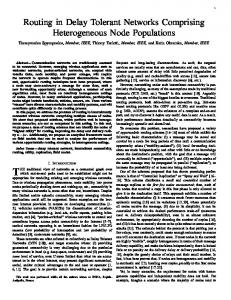
18 Oblivious (Dimension−Ordered) Routing

Adaptive Routing

Figure 1.1: Adaptive routing achieves better physical link utilization from oblivious routing. destination pair without taking into account the state of the network. The problem is illustrated in Figure 1.1. As can be seen from the gure, oblivious routing cannot achieve good physical link utilization because of strong restrictions in the use of physical channels. In Figure 1.1, three nodes try to send messages to three dierent destinations. Dimension-Ordered routing forces the messages to use the same physical channels, thus overloading the physical links and decreasing performance. Messages rst have to reduce their oset along x and then along y. Adaptive routing, on the other hand, is capable of assigning dierent paths between each source and destination based on channel availability. If a desired physical channel is busy, another channel leading towards the destination may be chosen. Adaptive routing algorithms can achieve a much better utilization of physical links and thus increase performance. A number of studies regarding the performance of adaptive routing have been published. Among those, we pick the one by Duato and Lopez [DL94] because the routing algorithm evaluated has been derived using the same methodology that will be used in chapter 4 to construct Adaptive Routing. This study examines a variety of trac patterns and also takes into account the fact that adaptive routers need more complicated routing logic than oblivious routers. This assumption is incorporated in the study in the form of increased cycle time for the adaptive router. Chien's parametric speed model [Chi93] was used to derive speci c cycle times. The results indicate that adaptive routing consistently produces lower average message latency than Dimension-Ordered routing for all trac patterns.

1.2. CONTRIBUTIONS OF THIS WORK

19

Adaptive routing has critics too. Recently, Pertel [Per92] has published a study in which he presents simulation results that allegedly refute the claims that adaptive routing is superior to Dimension-Ordered routing in terms of performance (average message latency). The main conclusion of the study is that under heavy trac, Dimension-Ordered routing tends to queue more packets at their source and fewer packets in the network compared to adaptive routing. Queueing in the network is the major factor that contributes to the increased message latency exhibited by adaptive routing. There are two main issues that undermine the signi cance of Pertel's results: 1. All results assume random uniform trac patterns. There is no reason that adaptive routing should perform better in such cases. 2. Pertel's simulator assumes in nite buering to resolve deadlocks in adaptive routing. This is not a realistic assumption. In nite buering practically eliminates backpressure at the source and can increase unrealistically network queue sizes. Given this assumption, Pertel's conclusion regarding network queue sizes is self-induced. Adaptive routing is a very promising approach to take advantage of the rich and regular connectivity of multicomputer networks. Increasing the utilization of the network bisection bandwidth will increase performance in most trac cases. The only serious disadvantage of adaptive routing is the design complexity introduced to the switching element.

1.2 Contributions of this work A number of wormhole adaptive routing algorithms have appeared in the literature [NM93]. Yet, there are no hardware implementations of such algorithms in part because of the diculty and design complexity involved. This thesis presents a complete solution to the problem of adaptive routing ranging from the formal de nition of a simple but powerful routing algorithm to the circuit implementation and layout. The algorithm presented is fully adaptive, can handle a single non-transient fault at a time, and has advanced features such as neighbor routing if the original message recipient is not available due to a fault. The circuit presented has a worst case delay of 6 ns (slowest process corner) when implemented in the hp26 process, and has a total area of 236m  904m.

20

CHAPTER 1. INTRODUCTION

1.3 Thesis Overview Chapter 2 gives some background information on adaptive routing. It presents adaptive routing algorithms proposed in the current literature and brie y analyzes their strong and weak points. Chapter 3 presents a number of formal de nitions regarding interconnection networks, routing functions and dependencies between virtual channels. It also presents two important theorems, the rst by Dally [DS87] and the second by Duato [Dua93] regarding deadlockfreedom in wormhole networks. Chapter 4 formally de nes Adaptive Routing, an adaptive routing algorithm for k-ary n-meshes. It also proves that Adaptive Routing is deadlock-free. Chapter 5 augments the Adaptive Routing algorithm presented in the previous chapter with the capability to handle a single non-transient fault at a time anywhere in the network without interruption of service. The resulting algorithm is called Reliable Adaptive Routing. The chapter also includes a proof of deadlock freedom. Chapter 6 describes the Virtual Channel Dependency Analyzer (VCDA). The VCDA is a software tool that helps in the visualization and analysis of Reliable Adaptive Routing. It can also prove by exhaustion that Reliable Adaptive Routing is deadlock-free. Chapter 7 is concerned with implementation issues. It describes the physical design of a two-dimensional version of Reliable Adaptive Routing. The resulting circuit is actually used in the MIT Reliable Router [DDH+94b], a high-performance network switching element. Chapter 8 describes how the circuit presented in the previous chapter ts into the Reliable Router design. Moreover, it presents a message retransmission mechanism which must be used in conjuction with adaptive routing for a reliable network layer. Finally, Chapter 9 summarizes and conludes the document.

Chapter 2

Background This chapter constitutes a survey of wormhole adaptive routing algorithms for low dimensional bidirectional meshes that have appeared in the literature. A brief overview of each algorithm is presented along with a discussion of strong and weak points. The rst section of the chapter introduces a common study framework in terms of a number of evaluation criteria. These criteria are mainly concerned with the degree that a routing algorithm can be easily and eciently implemented in a VLSI system.

2.1 Evaluation Criteria Reasonable Virtual Channel Requirements Virtual channels [DS87] can be very

expensive to implement. Not only do they require additional on-chip memory, but also they require allocation mechanisms and arbitration layers for other resources that are shared among them. Chien [Chi93] presents a parametric model that quanti es the cost of virtual channels in a generic router architecture in terms of number of gates and added latency. Virtual channels in adaptive routing algorithms are used to guarantee deadlock-freedom. We are interested in adaptive routing algorithms that require a small number of virtual channels in order to be deadlock-free.

Minimality A routing algorithm is minimal if it does not allow misrouting steps { steps

that will move a message away from its destination. Minimality is important for two reasons: First, it guarantees freedom from livelock. Second, it prevents wasting network resources in terms of channels and buers used to take a message further from its destination [Dal90]. Minimality is a desirable property in a routing algorithm. Departures from minimality should only take place when there is absolutely no alternative due to a faulty link. 21

CHAPTER 2. BACKGROUND

22

Full Adaptivity Full adaptivity means that a routing algorithm gives maximum routing freedom (within the limits placed by minimality) to a message trying to reach its destination. A fully adaptive algorithm can assign a next step channel of any possible direction that will move the message one step closer to its destination. Full adaptivity is a desirable property because more choices result in increased performance for non-uniform trac patterns.

Fault Tolerance Fault-tolerance is the ability of a routing algorithm to bypass faulty

links in the network. We are interested in routing algorithms that can handle gracefuly one non-transient fault at a time anywhere in the network.

Dependence on Local Information This last requirement means that the routing de-

cision depends only on the current position of a message and the position of the message destination. It does not depend on any past routing decisions. This requirement simpli es the physical design of the routing subsystem because it does not involve updating the header of a message with certain state information. Moreover, it makes possible to employ a higher level end-to-end error detecting (or correcting) protocol that includes the message header as well.

2.2 The Linder-Harden Algorithm Linder and Harden [LH91] have proposed a fully adaptive routing algorithm for bidirectional k-ary n-cubes. The main idea behind the Linder-Harden approach is the partitioning of the bidirectional physical network into several Virtual Networks. These virtual networks are unidirectional in all dimensions except for dimension 0. Messages are routed within a single virtual network throughout their course. The selection of the virtual network to be used by each message is based on the relative address of the message source with respect to the message destination. Routing within each virtual network is fully adaptive (minimal). Disadvantages of this algorithm are: 1. The Linder-Harden approach requires 2n?1 virtual networks where n is the dimension of the mesh, and therefore requires 2n?1 virtual channels per physical channel. The exponential dependence of the number of virtual channels on the mesh dimension makes the Linder-Harden algorithm impractical for network dimensions greater than two.

2.3. PLANAR ADAPTIVE ROUTING

23

2. The Linder-Harden scheme is not designed for fault-tolerance. Routing is minimal and does not allow side steps. Fault tolerant capabilities can be added in an ad hoc fashion on top of the existing algorithm at the expense of more virtual channels.

2.3 Planar Adaptive Routing Chien and Kim have proposed Planar Adaptive Routing [CK92]. Planar Adaptive Routing provides adaptivity in only two dimensions at a time. Figure 2.1 contrasts Planar Adaptive Routing with a fully adaptive routing algorithm in three dimensions. Within each adaptive plane, messages are routed in a fully adaptive fashion in a way very similar to the LinderHarden algorithm. More speci cally, in every adaptive plane Ai , the physical network is partitioned into two virtual networks: The increasing network which is used for messages that need to travel in the positive direction along dimension i, and the decreasing network, used by messages that need to travel in the negative direction along dimension i. When the distance in dimension i is reduced to zero, the message proceeds to adaptive plane Ai+1 . In the two-dimensional mesh case, Planar Adaptive Routing is equivalent to the Linder-Harden approach. By providing adaptivity to only two dimensions at a time, Chien and Kim have managed to reduce the virtual channel requirements of the Linder-Harden algorithm. Planar Adaptive Routing needs 3 virtual channels per physical channel for an n-dimensional mesh except for n = 2. In this case only two virtual channels are necessary. The Planar Adaptive Algorithm can be extended to handle faults that form convex regions within the network. The fault-tolerant version still requires 3 virtual channels per physical channel. The two-dimensional case requires 3 virtual channels as well. There are three major drawbacks in the way that the Planar Adaptive algorithm handles faults: 1. Misrouting steps result in tagging the message header. Therefore, the routing decision does not depend on local information only. 2. The algorithm requires an intermediate deactivation phase each time a fault occurs to ensure that the faulty regions are convex. In the case where there is a fault along the edge of the network, the deactivation algorithm will deactivate all k nodes along that particular edge. In conclusion, Planar Adaptive Routing is not an attractive routing algorithm because of limited adaptivity and complications and ineciencies in the fault-tolerant version.

CHAPTER 2. BACKGROUND

24

(a)

(b)

Figure 2.1: An example of Planar Adaptive Routing (a) vs. fully adaptive routing (b).

(a)

(b)

(c)

Figure 2.2: An illustration of the Turn Model in a 2D mesh: (a) abstract cycles in a 2D mesh; (b) four turns (solid arrows) allowed in Dimension-Ordered Routing; (c) six turns (solid arrows) allowed in West-First routing. This gure has been reproduced from Ni and McKinley [NM93]

2.4 The Turn Model For Adaptive Routing Glass and Ni have proposed the Turn Model for Adaptive Routing [GN92]. The Turn Model is an elegant framework that can produce a family of partially adaptive routing algorithms which have the highest possible degree of adaptivity that can be achieved using a single virtual channel. Deadlocks in wormhole routing are caused by messages waiting on each other in a cycle. The Turn Model prevents deadlocks by placing restrictions on the turns that a message can take throughout its course. The fundamental concept in this algorithm is the prohibition of the smallest number of turns so that cycles are prevented. Figure 2.2 illustrates the concept behind the Turn Model in a two-dimensional mesh. Figure 2.2 (a) shows the two abstract cycles that can cause deadlocks in a 2D routing algorithm. Figure 2.2 (b) shows the four turns that are prohibited in Dimension-Ordered routing. Finally 2.2 (c) shows that Dimension-Ordered routing places more restrictions than necessary for deadlock-freedom. The formation of cycles that lead to deadlock can be pre-

2.4. THE TURN MODEL FOR ADAPTIVE ROUTING

25

Figure 2.3: Example message paths under the West-First routing algorithm vented by prohibiting only two turns instead of four. The resulting routing algorithm that can be derived from the prohibition of the two turns in Figure 2.2 (c) is called West-First: It routes a message rst west if necessary and then it routes it nonminimally adaptively south, east and north. Example message paths under the West-First algorithm are shown in Figure 2.3. Other algorithms can be constructed by prohibiting a dierent pair of turns. Although the Turn Model is a simple and elegant framework for adaptive routing with minimal resource requirements, it has a number of weak points: 1. It does not scale easily to more than two dimensions. The framework with the abstract cycles does not extend in an obvious fashion to more than two dimensions because of the possibility of cycle formation that spans three or more dimensions. 2. The Turn Model produces algorithms that are not symmetric and place an uneven load on the physical links of the network. Independent studies by Glass and Ni [GN92] and Boppana and Chalasani [BC93] have concluded that the performance of Turn Model routing is inferior to other routing schemes especially for uniform trac. 3. The Turn Model does not produce fault-tolerant algorithms.

CHAPTER 2. BACKGROUND

26

2.5 Dimension Reversals Dally and Aoki [DA93] have proposed an adaptive routing algorithm which is based on the notion of \dimension reversals". Dimension reversals is the count of the number of times a packet has been routed from a channel in one dimension to another in violation of the dimension order imposed by the underlying Dimension-Ordered routing algorithm. The static version of the algorithm divides the virtual channels of each physical link into r classes where r is the maximum number of permitted dimension reversals. Messages with a dimension reversal count less than r can be routed adaptively but only using channels of class equal to their dimension reversal count. Once a message has a dimension reversal count equal to r it can only be routed using Dimension-Ordered routing on virtual channels of class r. The dynamic version of the algorithm does not place an upper bound on the dimension reversal count. It divides the virtual channels of each physical channel into two classes: adaptive and oblivious. Messages originate in adaptive channels. While in those channels messages can be routed along any direction. The dimension reversal count is maintained in the same way as before. Each time a virtual channel is allocated to a message, it is marked with the dimension reversal count of the message. To avoid deadlock, a message may not use a channel labeled with a count less than or equal to its own dimension reversal count. If an appropriate adaptive channel is not found, the message switches to the oblivious channels under Dimension-Ordered routing. It may not reenter the adaptive channels. This routing scheme is not attractive for a number of reasons: 1. Updating dimension reversal counts and marking virtual channels increases routing complexity signi cantly and does not meet the requirement that the routing decision should depend on local information only. 2. The algorithm is not fault-tolerant.

2.6 Compressionless Routing Kim, Liu and Chien have recently proposed Compressionless Routing [KLC94]. The main concepts behind this scheme are: Compressionless Routing (CR) supports deadlock recovery instead of prevention because according to the authors deadlocks are infrequent. Second, CR uses the feedback that wormhole routing provides in the form of ow control.

2.7. PIPELINED CIRCUIT SWITCHING

27

A message routed under Compressionless Routing does not release intermediate virtual channel buer storage until the head it reaches its destination. In this way, the tail it of the message does not leave the source node before the head it reaches the destination. If the message length is shorter than the distance between the message source and destination, then the message is padded with idle its to ensure that the message header reaches the destination before the last it has been injected by the source. The sender keeps track of the number of its it has injected, and increments a timeout counter each time that it cannot inject a it. The timeout counter is reset each time a it is injected. After a number of its equal to the distance between the source and the destination have been injected, the sender releases the path because the header has succesfully reached the destination and there is no possibility for deadlock. If on the other hand, the timeout counter reaches a threshold value before the header reaches the destination, then this indicates a possible deadlock. In such a case, the sender tears down the connection and will attempt retransmission after a certain time period. Since this scheme supports deadlock recovery instead of prevention, routing is fully adaptive with no restrictions and no virtual channels. Compressionless Routing can be thought of as a recast of circuit switching adapted to wormhole networks. Compressionless Routing can have serious performance problems: 1. CR is an unstable routing scheme because it resolves con icts by dropping [Dal90]. This means that for trac over a certain threshold, network throughput will drop dramatically. 2. CR is geared to small it size, small physical channel bandwidth and very narrow it buers in each network node. Unless the above are true, sending medium and short messages under Compressionless Routing will result in sacri cing substantial network bandwidth due to message padding.

2.7 Pipelined Circuit Switching Another similar approach to Compressionless Routing is Pipelined Circuit Switching (PCS) proposed by Allen, Gaughan, Schimmel and Yalamanchili [AGSY94]. PCS has been implemented in hardware in the Ariadne Router. PCS is dierent from wormhole routing in the following respect: In wormhole routing, data its immediately follow the head it in a pipeline fashion. In PCS, the data its do

CHAPTER 2. BACKGROUND

28

not immediately follow the head it into the network. Instead, the head it acts as a probe that sets up a circuit. When the head reaches the destination, an acknowledgment returns to the source. Only then can the data its be pipelined through the circuit that has been set up. The fact that the data its do not immediately follow the head it results in increased

exibility in the routing of the head. The head it can backtrack and release previously reserved virtual channels instead of blocking and waiting on busy channels. PCS can use the family of Misrouting-Backtracking (MB-x) protocols [GY93] for head it routing. The MB-x protocols search the network for a path in a depth- rst manner. Routing is minimal with the addition of x misrouting steps. The misrouting count is decremented each time a misrouting step is reversed. Neither deadlock nor livelock can occur because MB-x protocols do not block holding resources and they can use history information to avoid searching the same path repeatedly. PCS uses three virtual channels per physical channel. Data and control information (header) use separate virtual channels. There is an extra virtual channel that has the opposite direction from the previous two and is reserved for backwards-travelling its: acknowledgments and backtracking its. There are three main concerns with PCS: 1. The added round trip probe latency will have a big impact on network performance. 2. Maintaining misrouting history for a number of misrouting steps greater than one can sunstantially increase system complexity. 3. There is no support for fault tolerance once the circuit has been set up.

2.8 -cube3 Algorithm f

An interesting fault-tolerant extension to e-cube (Dimension-Ordered) routing was recently proposed by Boppana and Chalasani [BC94]. Faults are grouped into fault sets that occupy rectangular regions such that the boundary of the rectangle has only fault-free nodes and channels and the interior of the rectangle contains all the faulty channels and nodes that correspond to that particular fault set. This fault model is superior to the convex fault regions proposed by Chien and Kim [CK92] because it deals more eectively with faults along the network boundary. Boppana and Chalasani develop the concept of fault rings

2.8. F-CUBE3 ALGORITHM

29

FAULT CHAIN

FAULT RINGS

Figure 2.4: Fault chains and fault rings in f-cube3 routing. This gure is reproduced from Boppana and Chalasani [BC94]. and fault chains, rectangular paths around the fault regions that consist of fault-free nodes and links. Figure 2.4 shows examples of such structures. Messages are routed under regular Dimension-Ordered routing until they reach a fault ring or a fault chain. Then, depending on the relative position of the destination, messages are routed clockwise or counterclockwise around the fault ring until all misrouting steps are reversed. Three virtual channels are necessary to ensure deadlock-freedom. The disadvantages of this algorithm are: 1. f-cube3 is not an adaptive routing algorithm. Although it requires a minimum of three virtual channels for deadlock freedom, it is a fully oblivious scheme. Adaptivity can be added on top of the underlying fault-tolerant algorithm at the expense of more virtual channels. 2. f-cube3 requires a cumbersome setup phase each time a fault occurs during which nodes around the fault exchange messages to determine their position on the fault ring. Such a phase can add considerable complexity to the system. Moreover, f-cube3 requires updating the message header to indicate misrouting and direction around the fault ring. 3. Overlapping fault rings cannot be handled in f-cube3. Extra virtual channels are necessary for deadlock-freedom.

CHAPTER 2. BACKGROUND

30

Algorithm VC's (min) Adaptivity Minimality Local Info Linder-Harden 2n?1 Full Yes Yes Planar Adaptive 3 Partial Yes Yes Turn Model 1 Partial No Yes Dimension Reversals (s) r Full Yes No Dimension Reversals (d) 2 Full Yes No Compressionless 1 Full Yes Yes PCS 3 Full No No f-cube3 3 None Yes No Duato's New Theory 2 Full Yes Yes Table 2.1: A brief comparison of existing adaptive routing algorithms (a)

2.9 Duato's New Theory on Adaptive Routing Duato [Dua91][Dua93] has set up a theoretical framework and provided a methodology for constructing fully adaptive routing algorithms with minimal virtual channel requirements. Duato divides the virtual channels of each physical channel in two classes: oblivious and adaptive. Messages can use both channel classes and switch freely between the two. Duato studies the dependencies among the oblivious channels. Part of these dependencies are direct dependencies and are introduced by messages using two consecutive oblivious channels, and the rest of the dependencies are indirect and are introduced by messages using oblivious channels, then switching to adaptive and then switching back to oblivious. Duato proves that such an adaptive routing algorithm is deadlock-free if there are no cyclic direct nor indirect dependencies. The minimum number of virtual channels necessary for algorithms derived using Duato's methodology is two. Duato's methodology is valuable because it can be used to add full adaptivity on top of an existing deadlock-free oblivious routing algorithm at the expense of one more virtual channel.

2.10 Summary and Conclusion This chapter has presented a number of wormhole adaptive routing algorithms that have appeared in the literature. Tables 2.1 and 2.2 summarize the algorithms presented in terms of the evaluation criteria set in section 2.1. As one can see from the tables, none of the proposed algorithms is particularly attractive either because it does not meet our criteria or because it does not have adequate performance. Of all the algorithms presented, Duato's

2.10. SUMMARY AND CONCLUSION Algorithm Linder-Harden Planar Adaptive Turn Model Dimension Reversals (s) Dimension Reversals (d) Compressionless PCS f-cube3 Duato's New Theory

31

Support for Fault Tolerance Ad hoc and not well integrated Inecient and complicated because of deactivation algorithm. Incomplete Incomplete Incomplete Complete but decreases performance Incomplete Complete but complicated Left to designer

Table 2.2: A brief comparison of existing adaptive routing algorithms (b) theory and methodology is the most attractive candidate. In the next chapters we will use Duato's theory to construct a new fault-tolerant adaptive routing algorithm which meets all the requirements set in section 2.1. We call this algorithm Reliable Adaptive Routing.

Chapter 3

De nitions, Theorems and Notation This chapter presents a number of de nitions necessary for clarity and coherence throughout this document. Two very important theorems are also presented which will serve as the basis for the proof that the routing algoritm presented in Chapter 5 is deadlock-free. But rst the notation that will be used in subsequent chapters is introduced and explained.

3.1 Notation The following notation will be used throughout the rest of this document.

ca

src(ca ) dst(ca) x(ca ) y(ca )

A virtual channel. The source node of virtual channel ca. The destination node of virtual channel ca . The x address of src(ca). The y address of src(ca).

Figure 3.1 can be a helpful reference for the notation used.

3.2 De nitions The de nitions that appear in this section are based on the de nitions given by Dally [DS87] and Duato [Dua93].

De nition 1 An interconnection network I is a strongly connected directed graph, I =

G(N; C ). The vertices of the graph N represent the set of processing nodes. The arcs of 32

3.2. DEFINITIONS

33 src(Ca)

dst(Ca)

Ca 10

11 X(Ca) = 1 Y(Ca) = 0

Figure 3.1: Notation used. the graph C represent the set of communication channels. More than one arcs may connect two nodes.

De nition 2 A routing function R  C  N  C p where p is an integer, maps the current channel cc and the destination node nj to a set of channels where the packet can be routed next.

De nition 3 A routing subfunction R for a given routing function R and channel subset C  C , is a routing function such that: 1

1

R1 : C  N  C1p j R1(c; n) = R(c; n) \ C1p 8c; n 2 (C; N )

(3:1)

where p again is a positive integer.

De nition 4 A channel dependency graph D for a given interconnection network I and a routing function R, is a directed graph, D = G(C; E ): The vertices of D are the channels of I . The edges of D are the pairs of channels connected by R:

E = (ci; cj ) j cj 2 R(ci ; n) for some n 2 N:

(3:2)

De nition 5 Given an interconnection network I , a routing function R, a channel subset C  C which is the range of a routing subfunction R , a channel cs and a pair of channels ci ; cj 2 C , there is a direct dependency from ci to cj if 1

1

1

ci 2 R(cs; n) cj 2 R(ci; n)

(3.3) (3.4)

34

CHAPTER 3. DEFINITIONS, THEOREMS AND NOTATION These channels belong to channel subset C−C1

These channels belong to channel subset C1

Ci

C1

C2

C3

Ck

Cj

Indirect Dependency from Ci on Cj

Figure 3.2: Visualizing Indirect Dependencies. In other words, cj can be used immediately after ci by messages travelling from channel cs to a destination node n.

De nition 6 Given an interconnection network I , a routing function R, a channel subset C  C which is the range of a routing subfunction R and a pair of channels ci; cj 2 C , 1

there is an indirect dependency from ci to cj i

1

8 > c 2 R (c ; n) > < c1i 2 R1(ci;i?n1) 9c1; c2; : : :; ck 2 C ? C1 j > c 2 R(c ; n) m = 1, : : : , k - 1 > : cmj 2+1R1(ck ; mn) for some n 2 N

1

(3:5)

Figure 3.2 can be helpful in understanding better the de nition of an extended dependency. The existence of an indirect dependency between channels ci and cj means that it is possible to establish a path from ci to dst(cj ) where ci and cj are the rst and last channels of the path and belong to channel subset C1 and all the intermediate channels belong to channel subset C ? C1.

De nition 7 An extended channel dependency graph DE for a given interconnection net-

work I and routing subfunction R1 of a routing function R, is a directed graph, DE = G(C1; EE). The vertices of DE are the channels which are the range of the routing subfunction R1. The arcs of DE are the pairs of channels (ci ; cj ) such that there is either a direct or indirect dependency from ci to cj .

3.3. THEOREMS

35

3.3 Theorems Theorem 3.1 (Dally) A routing function R for an interconnection network I is deadlock-

free if there are no cycles in the channel dependency graph D.

Dally [DS87] presents a formal proof of this theorem. Duato [Dua93] presents a slightly dierent version of the proof.

Theorem 3.2 (Duato) A routing function R for an interconnection network I is deadlockfree if there exists a subset of channels C  C which forms the range of a routing subfunc1

tion R1 which is connected and has no cycles in its extended channel dependency graph DE .

Duato [Dua93] has formally proved the above theorem. Theorem 3.2 has shown that Theorem 3.1 imposes too strong a constraint on a routing function R in order to be deadlockfree: The acyclic channel dependency graph is a sucient but not a necessary condition. Theorem 3.2 poses a less strong constraint on R. The result is that \cheaper" adaptive routing algorithms can be made now possible (in terms of the number of virtual channels necessary to ensure freedom from deadlock.) Actually, both Theorems 3.1 and 3.2 only give a necessary but not sucient condition for a routing function R to be deadlock-free. Duato [Dua94a] has showed that the inverse of Theorem 3.2 is not true and the necessary condition is not as strong as the one suggested in the above theorem. Yet, Theorem 3.2 is sucient for the development of a simple and symmetric fault-tolerant adaptive routing algorithm which can be easily implemented in silicon. This theorem will be used to show that the algorithm presented in the following chapters is deadlock-free. There is a dierence in the de nitions given by Duato for a routing function and a routing subfunction and the de nitions presented in the previous section. Duato [Dua93] de nes a routing function as follows:

R : N  N 7! C p

(3:6)

We have decided to de ne a routing function as Dally [DS87] does.

R : C  N 7! C p

(3:7)

Duato does not de ne a routing function as in Equation 3.7 because in such a case Theorem 3.2 would not be valid. Consider for example two subsets of C , C1 and C ? C1.

36

CHAPTER 3. DEFINITIONS, THEOREMS AND NOTATION

Let R be a routing function de ned in such a way that all messages arriving in a node through a channel that belongs to the C ? C1 subset are routed to a channel that belongs to the same subset. Suppose that are cyclic dependencies among the channels that belong to C ? C1. Moreover, suppose that there exists a routing subfunction R1 whose range is C1. R1 is connected and has no cycles in its extended channel dependency graph. In such a case, R is not guaranteed to be deadlock-free. We believe it is important make the domain of a wormhole routing function C  N instead of N  N for the following reasons: 1. As Dally [DS87] suggests, the formulation of routing as a function from C  N to C p has more memory than the conventional de nition of routing as a function from N  N to C p . This de nition has actually helped to develop the notion of channel dependence. 2. The formulation from C  N to C p provides information that is actually used in certain cases by the algorithm to be described in the following chapters. As an example, our algorithm does not allow the use of C ? C1 channels when some conditions hold, one of which is that the message arrives at the node through a C1 channel. A de nition such as 3.7 is most appropriate in such cases. In order to make Theorem 3.2 valid and still maintain C  N as the domain of the routing function we need to impose one constraint on R. Given a routing function R : C  N 7! C p, a channel subset C1 and a routing subfunction R1 : C  N 7! C1p, Theorem 2 is valid if

R(c; n) \ C1p 6= ; 8(c; n) 2 C  N

(3:8)

In other words, R is de ned in such a way that it is never possible for a message to be forced to use only C ? C1 channels after a certain point in its course. If this provision is met, the pathological case described above will be avoided.

Chapter 4

Adaptive Routing This chapter presents an adaptive routing algorithm with a minimum number of virtual channels. This algorithm does not have fault-handling capabilities. We name this algorithm Adaptive Routing (AR) as opposed to Reliable Adaptive Routing (RAR) which will be presented in the next chapter. This particular choice of presentation was made because an incremental approach is easier to organize and easier to be understood and appreciated by the reader.

4.1 Informal Description AR needs two virtual channels per physical channel to ensure that there will be no deadlocks. AR is minimally adaptive: A message can only make steps that will bring it closer to its destination (productive). Unproductive steps (misrouting) are not allowed. One of the two virtual channels is the Adaptive channel and the other is the DimensionOrdered channel. When a message gets injected into the network, it starts to route on the Adaptive channels. AR can assign any free productive Adaptive channel as a possible next step. A virtual channel is considered free if it is currently not allocated to a message. If there are no free Adaptive channels AR assigns the unique Dimension-Ordered virtual channel that corresponds to the current position of the message and its destination. This unique Dimension-Ordered virtual channel is the same one as the one that would be assigned by a pure Dimension-Ordered routing function given the current message position and the message destination. If after the next hop there are free Adaptive channels, the message switches back to them. A Dimension-Ordered routing function routes messages in strict dimension order: In every dimension d a message is routed along that dimension until it reaches a node whose address 37

CHAPTER 4. ADAPTIVE ROUTING

38

Z

Y X

(a)

(b)

Figure 4.1: Minimally Adaptive Vs. Dimension-Ordered Path. in dimension d matches the address of the message destination in the same dimension. If the addresses match, then the packet continues to route in the next lower dimension d ? t; t > 0 where the current channel address and the destination address dier. Figure 4.1 contrasts a minimally adaptive vs. a dimension-ordered message path in a 3-dimensional mesh. The order of dimensions in this case is fx,y,zg. Dimension-Ordered Routing even with a single virtual channel per physical channel (assuming that the network is not toroidal and there are no wraparound paths) has been proven to be deadlock-free [DS87]. Figure 4.2 shows an example of a message path under AR. The message starts to route on Adaptive channels when it enters the network. It follows an adaptive minimal path. At some point in the path, no free Adaptive channels were available and AR started assigning Dimension-Ordered channels. While routing on Dimension-Ordered channels, the message had to match the x address of its destination before routing on the y dimension. Later in the course, Adaptive channels became available again, and the message reached its destination on Adaptive channels. Figure 4.3 shows a owchart of the routing algorithm. AR is deadlock-free. There are cyclic dependencies among the Adaptive channels. Yet, AR does not let a message block while waiting for an Adaptive channel to become free. The routing function assigns a Dimension-Ordered channel instead. There are no cyclic dependencies among Dimension-Ordered channels. As a result, messages can block on such channels without the risk of forming a deadlocked con guration.

4.1. INFORMAL DESCRIPTION

39

Adaptive Channels Dimension−Ordered channels

y

x

Figure 4.2: Example of a Path Under Adaptive Routing.

START

Have we reached the destination?

Yes

No Available

Route on a productive Adaptive Channel Not Available Route on unique DO channel

Figure 4.3: Flowchart of Adaptive Routing

END

CHAPTER 4. ADAPTIVE ROUTING

40

4.2 Formal Description This section will apply the de nitions and the theorems of the previous chapter on AR and give a formal proof that the algorithm is deadlock-free.

4.2.1 Notation Let x be an n-digit radix-k number. x will be represented as xn?1 xn?2 : : :xi+1 xi : : :x1x0 where xi < k; 8i 2 [0; n ? 1]. xi will denote the ith digit of x. Numbers in such a format will be used to indicate addresses in a k-ary n-cube interconnection network. The following notation will be used:

nx

Any node in a k-ary n-cube, where x is the node adress (n-digit radix-k number.) p(nx ) The consuming (processor) channel associated with node nx . ci i integer Any virtual channel. cai i integer An Adaptive virtual channel. cdi i integer A Dimension-Ordered virtual channel. free(cai ) 1 if channel cai is not allocated to a message, 0 otherwise. The subscript i of Adaptive and Dimension-Ordered channels cfa; dgi can be partitioned in a number of the form drfx where:

d the dimension of the channel. r the direction of the channel (1 increasing, 0 decreasing.) f productive routing indicator (k ? 1 ? xd for increasing channels, and xd for decreasing channels.)

x the network address of the channel source node (n-digit radix-k number.) Figure 4.4 shows the channel subscripts for all channels cdrfx in a 4-ary 2-cube.

4.2.2 De ning R and R

1

Channel sets C1 and C are de ned as follows:

C1 = fcdi; 8ig C = fci; 8ig = fcdi; 8ig [ fcai; 8ig C ? C1 = fcai ; 8ig

(4.1) (4.2) (4.3)

C is the set of all virtual channels in the network. C1 contains only the Dimension-Ordered channels and C ? C1 contains only the Adaptive channels.

4.2. FORMAL DESCRIPTION

41

11303 03

11213 13

10113

00303

01102

00313

10223

01112

11302 02

01201

00212

10222

01211

11301 01

01300

00111

10110

01132

32

00232

01231

11121 21

00121

10220

00333

10332

01221

10331

01320

11210 10

33

11122 22

00222

10221

01310

11300 00

01122

11211 11

10111

00101

00323

10333

11212 12

10112

00202

11123 23

31

00131

01330

11120 20

10330

30

Figure 4.4: Assignment of subscripts to channels in a 4-ary 2-cube. Let R1 : C  N 7! C1 be the function given by the following de nition:

R1(cddrfx; nj ) = 8 p(nj ) > > < cddr[f ?1][x?(?1)rkd ] cd 0 > r d > : cdd01[k?1?xd0 ][x?r (?d 1) k ] d 0[xd0 ][x?(?1) k

]

if 8m; [x ? (?1)r kd ]m = jm if [x ? (?1)r kd ]d 6= jd if (8m > d0 ; [x ? (?1)r kd ]m = jm ) ^ xd0 < jd0 if (8m > d0 ; [x ? (?1)r kd ]m = jm ) ^ xd0 > jd0

R1(cadrfx; nj ) = 8 > if 8m; [x ? (?1)r kd ]m = jm < p(nj ) if (8m > d0 ; [x ? (?1)r kd ]m = jm ) ^ [x ? (?1)r kd ]d0 < jd0 cd 0 r d > : cddd01[0[kx?01][?x?xd(0?][1)x?r k(?d ]1) k ] if (8m > d0 ; [x ? (?1)r kd ]m = jm ) ^ [x ? (?1)r kd ]d0 > jd0 d (4.4) For clarity purposes, the de nition of R1 has been broken in two parts: The rst part de nes R1 on domain C1  N while the second de nes it on (C ? C1)  N . The union of the two domains is C  N . Function R1 is nothing but the widely used dimensionordered routing function. This particular routing function routes in decreasing dimension

CHAPTER 4. ADAPTIVE ROUTING

42

order. This de nition is very similar to the one which Dally [DS87] de nes, but here it is augmented to accomodate bidirectional channels.

Assertion 4.1 The Channel Dependency Graph of routing function R is acyclic. 1

Proof It is evident from Equation 4.4 that R always assigns a virtual channel with a 1

decreasing subscript. More formally:

8ci; cj 2 C ; 8nc 2 N : 9R (ci; nc) = cj ) i > j: 1

1

(4:5)

Therefore, the Channel Dependency Graph is acyclic. 2 Let us consider a k-ary n-cube and a routing function Ra : C  N 7! (C ? C1)p given by the following de nition:

Ra(cdrfx; nj ) = fcad0r0 f 0x0 : free(cad0 r0 f 0 x0 ) = 1g

(4:6)

The subscript d0r0 f 0 x0 is given by the following equations:

6 jd0 d0 2 f0; 1; : : :; n ? 1g ^ [x ? (?1)r kd ]d0 = 8 > r d0 = d < 0 6 d ^ [x ? (?1)rkd]d0 > jd0 r = > 0 d0 = : 1 d0 6= d ^ [x ? (?1)r kd ]d0 < jd0 8 > d0 = d < f ?1 0 d0 6= d ^ [x ? (?1)r kd ]d0 > jd0 f = > xd0 : k ? 1 ? xd0 d0 = 6 d ^ [x ? (?1)r kd]d0 < jd0 x0 = [x ? (?1)r kd ]

(4.7) (4.8) (4.9) (4.10)

It is important to note that Ra can assign a set of possible channels for the next step in the message route. A selection function S : (C ? C1)p 7! C ? C1 will have to be applied to pick the single virtual channel on which the message will be routed next. S can be deterministic or stochastic and is of limited importance. In certain cases it is possible to have Ra = ;. This means that all the adaptive channels cai for some i are allocated to other messages. Although the de nition looks complicated, Ra is nothing but a minimal adaptive routing function. Equation 4.7 simply says that any channel can be assigned as a possible next step as long as it moves the message closer to its destination.

4.3. FACTS ABOUT R AND R1

43

We are now ready to de ne routing function R : C  N 7! C p.

8(c; n) 2 C  N R(c; n) = R (c; n) [ Ra(c; n)

(4:11)

1

Note that R1 is a subfunction of R by the de nition of Chapter 3.

4.3 Facts about R and R1 This section states and proves certain facts about functions R and R1 that will be used to prove that routing function R is deadlock-free.

Assertion 4.2 Let cdd fx and cdd f 0x0 be two Dimension-Ordered channels. There can be 1

0

no indirect dependency from cdd1fx on cdd0f 0x0 .

This assertion merely claims that there can be no indirect dependencies between two channels of the same dimension and opposite directions. If such a dependency exists, then this means that at least one of the intermediate adaptive (C ? C1 ) steps overshot the destination along the d dimension. More formally:

Proof Suppose that there exists an indirect dependency from channel cdd fx on channel 1

cdd0f 0x0 . Let cam1 ; cam2 ; : : :; camk be k intermediate adaptive channels. Moreover, let ng be the message destination. We have:

cam1 = S (Ra(cdd1fx; ng )) cam2 = S (Ra(cam1 ; ng )) cam3 = S (Ra(cam2 ; ng ))

.. . camk = S (Ra(camk?1 ; ng )) cdd0f 0x0 = R1(camk ; ng )

(4.12) (4.13) (4.14) (4.15) (4.16)

Since cdd1fx is a channel of positive direction, we know that:

xd < gd

(4:17)

CHAPTER 4. ADAPTIVE ROUTING

44

By directly applying de nition 4.6 on cdd1fx and the subsequent adaptive channels, we see that the following must be true:

dst(camk )d < gd

(4:18)

If the intermediate adaptive channels belong to dierent dimensions than d, then we see by 4.6 through 4.10 that this won't aect the dth digit of the destination node of each channel. Therefore the above equation holds. If on the other hand there are intermediate adaptive steps along the d dimension, then according to 4.6 through 4.10 this will increase the destination address by tkd where t is the number of steps along dimension d. In other words the dth digit of the destination will be increased by t radix-k units. In such a case the inequality may be converted to at most an equality: dst(camk )d = gd . Yet, this does not happen because if it did, the address of the destination along the d dimension would be matched and 4.4 cannot assign a dimension d channel as a possible next step route. Therefore 4.18 is valid in all the cases. Since 4.18 is true, de nition 4.4 will assign a channel cddrf 0 x0 with r=1. A channel cdd0f 0x0 cannot be assigned by routing function R1 and therefore no dependency may exist from cdd1fx and cdd0f 0x0 . 2 By symmetry arguments, the following assertion is also true:

Assertion 4.3 Let cdd fx and cdd f 0x0 be two Dimension-Ordered channels. There can be 0

1

no indirect dependency from cdd0fx on cdd1f 0x0 .

We can consolidate Assertion 4.2 and 4.3 into the following statement:

Assertion 4.4 Let cddrfx and cddrf 0x0 be two Dimension-Ordered channels. There can be no indirect dependency from cddrfx on cddrf 0 x0 .

Assertion 4.5 There is an indirect dependency from cdd fx on cdd f 0x0 if and only if xd < 1

x0d .

1

Proof If we proceed exactly the same way as we did for Assertion 4.2, then we have: x + kd < x0 ) xd < x0d:

2

(4:19)

4.3. FACTS ABOUT R AND R1

45

We also need to show the inverse. Let cdd1fx and cdd1f 0x0 be two Dimension-Ordered channels such that xd < x0d . Let g = dst(cdd1f 0x0 ). Without loss of generality let us assume that: 8i 2 [0; n ? 1] xi < gi (4:20) There exist adaptive channels such that:

ca01[k?1?(x+k0 )0 ][x+k0 ] = S (R(cd1fx; ng )) ca01[k?1?(x+2k0 )0 ][x+2k0 ] = S (R([
]; ng)) ca01[k?1?(x+(g0?x0 )k0 )0 ][x+(g0 ?x0 )k0 ] ca11[k?1?(x+k1 )1 ][x+(g0 ?x0 )k0 +k1 ] ca11[k?1?(x+2k1 )1 ][x+(g0?x0 )k0 +2k1 ] ca11[k?1?(x+(g1?x1 )k1 )1 ][x+(g0 ?x0 )k0 +(g1 ?x1 )k1 ]

.. . = = = .. . = .. . =

S (R([
]; ng)) S (R([
]; ng)) S (R([
]; ng)) S (R([
]; ng))

cad1[k?1?(x+kd )d][x+(g0 ?x0 )k0 +(g1 ?x1 )k1 +


+(gd?1 ?xd?1 )kd?1 +kd ] S (R([
]; ng)) cad1[k?1?(x+2kd)d][x+(g0?x0 )k0 +(g1 ?x1 )k1 +


+(gd?1 ?xd?1 )kd?1 +2kd ] = S (R([
]; ng))

.. . cad1[k?1?(x+(gd?xd +1)kd)d][x+(g0?x0 )k0 +


+(gd?1 ?xd?1 )kd?1 +(gd?xd +1)kd ] = .. . ca[n?1]1[k?1?(x+kn?1 )n?1 ][x+(g0?x0 )k0 +


+(gn?2 ?xn?2 )kn?2 +kn?1 ] = ca[n?1]1[k?1?(x+2kn?1 )n?1 ][x+(g0 ?x0 )k0 +


+(gn?2 ?xn?2 )kn?2 +2kn?1 ] = .. . ca[n?1]1[k?1?(x+(gn?1 ?xn?1 +1)kn?1 )n?1 ][x+(g0?x0 )k0 +


+(gn?1 ?xn?1 )kn?1 ] = cdd1f 0x0 =

S (R([
]; ng)) (4.21) S (R([
]; ng)) S (R([
]; ng)) S (R([
]; ng)) S (R([
]; ng)) (4.22)

In the above equations the running symbol [
] which appears in each equation refers to the left hand side of the previous equation. It is important to note that this particular choice of adaptive channels for the intermediate steps does not match the destination address

CHAPTER 4. ADAPTIVE ROUTING

46

along the d dimension (equation 4.21) so that the indirect dependency between cdd1fx and cdd10x0 may exist as indicated by equation 4.22 given our particular choice for the message destination. Therefore xd < xd0 constitutes both a necessary and sucient condition for an indirect dependency. 2 Using the same method, we can also prove the following statement:

Assertion 4.6 There is an indirect dependency from cdd fx on cdd f 0x0 if and only if xd > 0

x0d .

0

Assertion 4.7 If there is an indirect dependency from cddrfx on cdd0rf 0x0 and d0 6= d then d0 < d.

Proof Let cddrfx and cdd0rf 0x0 be two Dimension-Ordered channels such that there is an

indirect dependency from cddrfx on cdd0 rf 0 x0 . Let ng be the message destination. We know that cddrfx was the result of applying R1 on a channel ci such that dst(ci ) = x, and the message destination ng : R1(ci; ng ) = cddrfx (4:23) From de nition 4.4 we draw the conclusion that:

8d00 > d gd00 = xd00

(4:24)

In such a case equations 4.6 through 4.10 won't assign a channel of dimension d00 > d. Let caj be the last Adaptive channel used before cdd0rf 0 x0 . It must be that src(caj )d00 = gd00 8d00 > d. Application of R1 on (caj ; ng ) will therefore yield cdd0rf 0 x0 with d0 < d if d0 is to be dierent from d. 2

4.4 Proving Freedom from Deadlock We have a rich set of facts about routing functions R and R1. These facts can help us prove in a couple of steps that routing function R is deadlock-free.

Assertion 4.8 Let cddrfx; cdd0r0f 0x0 2 C be two Dimension-Ordered channels. If there 1

exists an indirect dependency from cddrfx to cdd0 r0 f 0 x0 then it must be that drfx > d0r0f 0 x0 .

4.4. PROVING FREEDOM FROM DEADLOCK

47

Proof There are two distinct cases. If d 6= d0 then from Assertion 4.7 we have d0 < d. Therefore drfx > d0 r0f 0 x0.

Now let us assume that r = 1. From Assertion 4.4 we know that r0 = r. If d = d0 then from Assertion 4.5 we have the following:

xd ?xd k ? 1 ? xd f drfx

< > > > >

x0d ?x0d k ? 1 ? x0d f0 d 0 r 0 f 0 x0

(4.25) (4.26) (4.27) (4.28) (4.29)

If r = 0 on the other hand (using Assertion 4.6) :

xd > x0d f > f0 drfx > d0r0f 0x0

(4.30) (4.31) (4.32)

And the proof is complete. 2 Finally we come to our conclusion:

Assertion 4.9 Routing function R is deadlock-free. Proof Let cdi; cdj 2 C be two Dimension-Ordered channels. If there is a direct depen1

dency from cdi to cdj then from Assertion 4.1 we know that i < j . If on the other hand there is an indirect dependency from cdi to cdj then from Assertion 4.8 we know that i < j . Therefore if there exists any dependency either direct or indirect from cdi to cdj it is true that i < j . Therefore, there are no cycles in the Extended Channel Dependency Graph of function R and by Theorem 3.2 R is deadlock-free. Before completing the proof we must make sure that condition 3.8 we have set is true:

R \ C1p = (R1 [ Ra) \ C1p = C1 6= ; This completes the proof. 2

(4:33)

48

CHAPTER 4. ADAPTIVE ROUTING

4.5 Summary In this chapter we have formally de ned a fully adaptive routing function R. R needs two virtual channels per physical channel, one Adaptive and one Dimension-Ordered. R makes messages follow minimally adaptive paths towards their destination. If Adaptive channels are not available at some step due to network contention, R will assign a Dimension-Ordered channel as the unique next step route. If Adaptive channels become free, then R will resume assigning Adaptive channels. We have stated and proven a number of facts about R which led us to the conclusion that R is deadlock-free by directly applying Duato's Theorem (3.2).

R is not fault-tolerant. In the next chapter we will augment R with the capability to

handle a single non-transient fault at a time anywhere in the network. A lot of the facts stated in this chapter will be used and exploited in the rest of this document.

Chapter 5

Reliable Adaptive Routing This chapter augments Adaptive Routing and enables it to handle a single link failure anywhere in the network, even along the edges. To achieve this, we need to introduce one more virtual channel per physical channel: The Fault-Handling channel. We call the resulting routing algorithm Reliable Adaptive Routing. The rst section will discuss the particular fault model assumed in the design of the algorithm. Next, an informal description of the algorithm will be given along with routing examples. Then, the algorithm will be formally de ned and nally a proof of deadlock-freedom will be presented.

5.1 Fault Model Our fault model is based on the following assumptions:

 We consider as fault a link failure anywhere in the network. A fault can be detected

by using parity or any other error detecting code on the wires of each physical link in the network.  Faults are non-transient. This means that as soon as a parity error is detected on a link, the link is agged as faulty(0). If the parity error is transient and goes away, the link status is not reset to 1. A link can only be returned to service through human intervention using a dedicated diagnostic port. Such an action does not disrupt the rest of the system.

 There can be only one fault at a time. Adaptive Routing as presented in the previous chapter cannot always assign a next step route in the presence of faults that conform to this model. Figure 5.1 shows two examples of such faults. 49

CHAPTER 5. RELIABLE ADAPTIVE ROUTING

50

Y

A

A

X

Figure 5.1: Faults that cannot be handled by Adaptive Routing. In both cases, the destination of the path is indicated by a white dot. In the rst case, a message has reached the y address of its destination through Adaptive channels and proceeds to reach the x address too through either Adaptive or Dimension-Ordered channels. There is a broken link in the way. Since R is a minimal adaptive function, the dotted path cannot be allocated and there is no way that this particular message will reach the destination. In such a case if c is the current virtual channel and n is the message destination, we have:

R(c; n) = ;

(5:1)

In the second example equation 5.1 will hold as well if the single eligible Adaptive channel that departs from node A (the y + channel) is busy. In both cases we see that R clearly needs to be augmented with the ability to assign paths such as the dotted paths shown in gure 5.1.

5.2 Informal Description This section will give an informal description of Reliable Adaptive Routing. RAR is almost the same with Adaptive Routing. The only dierence is that RAR provides an extra class of virtual channels to accomodate paths such as the dotted paths of Figure 5.1.

5.2.1 Examples First, we will describe RAR through some examples. The following examples assume that the dimension order assumed by routing function R1 (4.4) is fx,yg. In other words x is

5.2. INFORMAL DESCRIPTION

51

dimension 1 and y is dimension 0. Figure 5.2(a) shows an example of routing around a fault that occurs along the x dimension. In such a case, when the message is in node A, RAR will assign the dotted Fault-Handling channel and allow the message to take a nonminimal side step. After the side step has been taken, the message can continue to use Dimension-Ordered or Adaptive channels as it did before. In this case, the side step was taken along the y dimension. Since this constitutes a misrouting step, we know that it has to be reversed in the future. As we can see from Figure 5.2(a), this step is reversed just before the message reaches its destination. Reversing the misrouting step does not introduce any extra dependencies among C1 channels. Reversing the step involves a step from an x channel to a y channel. Such a dependency already exists in the Extended Channel Dependency Graph of routing function R. This is the rationale behind allowing the message to use Dimension-Ordered channels after it has used the Fault-Handling channel: No additional dependencies are created and therefore no deadlock is introduced. Case (b) is very similar to case (a) in that the message can continue to use DimensionOrdered channels after routing on a Fault-Handling channel without introducing extra dependencies. On the other hand, when the fault occurs along the y dimension as shown in Figure 5.2(c)(d) things are dierent. In this case the misrouting step has to occur along the x dimension which is a higher dimension than the one we are currently routing on. If this misrouting step is reversed on Dimension-Ordered channels, then additional dependencies must be added to the Extended Channel Dependency Graph from Dimension-Ordered y channels to Dimension-Ordered x channels. Such an action introduces potential deadlocks.

5.2.2 The Algorithm An informal de nition of Reliable Adaptive Routing follows: 1. First nd a free and non-faulty Adaptive channel which brings the message closer to its destination. 2. If such a channel is not found, nd the unique Dimension-Ordered channel that corresponds to the current channel position of the message and its destination. 3. If the unique Dimension-Ordered channel is not available due to a fault, then nd a productive Fault-Handling Channel.

CHAPTER 5. RELIABLE ADAPTIVE ROUTING

52

A

A

(a)

(b)

Y A

(c)

A

(d)

X

Figure 5.2: Faults handled by Reliable Adaptive Routing.

5.3. FORMAL DEFINITION

53

4. If a productive Fault-Handling channel is not available because the destination address only diers in a single dimension from the current address then if the unmatched dimension is dierent from dimension 0 do the following steps: (a) Route on an unproductive Fault-Handling channel along a dimension lower from the single unmatched dimension at this time. (b) Resume routing from step 1. If on the other hand, the unmatched dimension is 0 execute the following steps: (a) Route on an unproductive Fault-Handling channel along dimension 1. (b) Route on productive Fault-Handling channels along dimension 0 until the address of the destination in dimension 0 is reached. (c) Route on the Fault-Handling channel along dimension 1 which will bring the message to its nal destination. The algorithm described above is capable of assigning channels that form the message paths shown in Figure 5.2. We see that RAR can bypass a fault even if the fault occurs along the edges of the network. A owchart of the Reliable Adaptive Routing algorithm is shown in Figure 5.3.

5.3 Formal De nition This section presents a formal de nition of the routing algorithm that has been described in the previous section.

5.3.1 Notation The notation of section 4.2.1 will be used along with the following additions:

cfi

A Fault-Handling virtual channel. valid(ci ) 1 if channel ci is in service, 0 if it is faulty.

5.3.2 De ning R and R

2

Proof of deadlock freedom will be based again on Theorem 3.2. We need to rede ne routing function R and de ne a routing subfunction R2 with range C2 so that the requirements of

CHAPTER 5. RELIABLE ADAPTIVE ROUTING

54

START

Have we reached the destination?

Yes

END

No Route on a productive Adaptive Channel

Available

Not Available Available

Route on unique DO channel

Not Available Available

Route on productive FH channel

Not Available

No

Is the only remaining dimension to be matched 0?

Route on unproductive FH channel on dimension lower from single unmatched dimension

Yes

Route on unproductive FH channel along dimension 1

Yes

Is the only remaining dimension to be matched 1?

Route on productive FH channel along dimension 0 (one step remaining)

No

Route on productive FH channel along dimension 0

END

Figure 5.3: Flowchart of Reliable Adaptive Routing

5.3. FORMAL DEFINITION

55

the theorem are satis ed. Channel sets C2 and C are de ned as follows:

C2 = fcdi; 8ig [ fcfi; 8ig C = fci; 8ig = fcdi; 8ig [ fcai; 8ig [ fcfi ; 8ig C ? C2 = fcai; 8ig

(5.2) (5.3) (5.4)

C is again the set of all virtual channels in the network. C2 contains the DimensionOrdered channels and the Fault Handling channels. C ? C2 contains only the Adaptive

channels. The Fault-Handling channels must be included in channel subset C2 because subset C2 must be connected for Theorem 3.2 to be valid. Let R1 be the function de ned in 4.4. Routing function R2 will be de ned on two disjoint domains for reasons of clarity and simplicity. Let cfa; dgdrfx indicate an Adaptive or Dimension-Ordered channel. R2 de ned on such channels is given by the following de nition: ( R1 (cfa; dgdrfx; nj ) if 9c 2 R1 : valid (c) = 1 (5:5) R2(cfa; dgdrfx; nj ) = cf 0 0 0 0 otherwise drfx

Subscripts d0; r0; f 0; x0 are given by the following equations:

d0 f0

8 > dp 9dp; dp0 : [x ? (?1)r kd ] 0g 6= jfdp;dp0g ^ dp 6= dp0 > < du 9d00; d000 : [x ? (?1)r kd ]ffddp;dp 00;d000 g 6= jfd00 ;d000 g ) d00 = d000 = > 00 ^ 9du : du < d > : 1 otherwise ( [x ? (?1)r kd ]d0 > jd0 xd0 = k ? 1 ? x 0 [x ? (?1)r kd] 0 < j 0

x0 = x ? (?1)rkd

d

d

d

(5.6) (5.7) (5.8)

When R2 is de ned on Fault-Handling channels, it is given by the following de nition: 8 > p(nj ) if 8m; [x ? (?1)r kd ]m = jm > > R1(cddrfx; nj ) j[x ? (?1)r kd]1 ? j1j =6 1 > < cf01[k?1?x0 ][x?(?1)r kd ] j[x ? (?1)r kd ]1 ? j1j = 1 ^ x0 < j0 R2(cfdrfx; nj ) = > cf j[x ? (?1)r kd]1 ? j1j = 1 ^ x0 > j0 00x0 [x?(?1)r k d ] > > cf11[k?1?x1 ][x?(?1)r kd ] j[x ? (?1)r kd]1 ? j1j = 1 ^ x0 = j0 ^ x1 < j1 > : cf10x [x?(?1)r kd ] j[x ? (?1)r kd]1 ? j1j = 1 ^ x0 = j0 ^ x1 > j1 1 (5:9)

CHAPTER 5. RELIABLE ADAPTIVE ROUTING

56

B

A

D

Figure 5.4: Undesirable minimal step Let Ra2 be a minimal adaptive routing function much like the one de ned in 4.6 through 4.10. One dierence between Ra and Ra2 is shown in the following equation.

Ra2(cfa; d; f gdrfx; nj ) = fcai : cai 2 Ra(cfa; dgdrfx; nj ); valid(cai) = 1g

(5:10)

It simply says that the minimal adaptive function Ra2 can only pick channels that are not faulty. Except for this trivial constraint, there is an additional one which stems from the fact that misrouting steps are now possible: If no further constraints are imposed to the minimal adaptive routing function, then an undesirable situation may occur just after a misrouting step. This is illustrated in Figure 5.4. Suppose that a message misroutes due to a fault because the address of its current channel diers from the destination address in only one dimension. When the head of the message reaches node B, then the minimal adaptive routing function as de ned in Equations 4.6 through 4.10 and Equation 5.10 may immediately reverse the misrouting step and direct the message back to node A (node D in the Figure indicates the message destination.). This is clearly undesirable. We therefore need to place extra restrictions on the minimal adaptive routing function so that misrouting steps are not immediately reversed. We can formulate this as follows: The minimal adaptive routing function Ra2 may not assign a next step channel of the same dimension but opposite direction when the message reaches the node from Fault-Handling channels. More formally:

Ra2(cfdrfx ; nj ) = Ra(cfa; dgdrfx; nj ) ? fcadrf 0 [x?(?1)r kd] g where f 0 is given by the following equation: ( 0 0 f = kxd? 1 ? x rr = = 1 d

(5:11)

(5:12)

5.4. FACTS ABOUT RELIABLE ADAPTIVE ROUTING

57

Now that we have all the routing subfunctions of R we are one step away from the de nition of Reliable Adaptive Routing:

8(c; n) 2 C  N R(c; n) = R (c; n) [ Ra (c; n) 2

2

(5:13)

From the de nitions of R2 and Ra2 it is evident that de ning a routing function on domain C  N instead of N  N has been necessary for de ning Reliable Adaptive Routing without resorting to other non-elegant schemes that would allow us to provide the routing function with some sort of memory. Reliable Adaptive Routing makes use of the fact that an incoming message comes in from Fault-Handling channels. The next step assignment depends on the channel kind of an incoming message. Yet, RAR does not require modi cation of the header or any other message state. The routing decision as can be seen from the previous de nitions depends only on local information. Never does the routing decision depend on a past routing event. This greatly simpli es the implementation of the algorithm and reduces system complexity.

5.4 Facts About Reliable Adaptive Routing Before proceeding with the proof of deadlock freedom it is worthwhile to examine the properties of the Fault-Handling channels that are added to the C1 channel subset. Clearly, the Fault-Handling channels form an independent virtual network on top of the Adaptive and the Dimension-Ordered virtual networks that already exist. Yet, we do not wish to adopt this point of view for two reasons: 1. Not all Fault-Handling channels are actually used by the routing algorithm. There is one Fault-Handling channel per physical channel. Yet, the Fault-Handling channels that can actually be assigned by the routing algorithm are very limited, given that there can be only one fault at a time. 2. The Fault-Handling channels must be viewed as an addition to the Dimension-Ordered virtual network for restoring connectivity. This is the only approach that will allow us to use Duato's theorem to justify the claim that Reliable Adaptive Routing is deadlock-free. The location and number of Fault-Handling channels depends directly on the location of the fault within the network. We are exploring this issue in the following sections.

58

CHAPTER 5. RELIABLE ADAPTIVE ROUTING

Figure 5.5: Addition of Fault[Handling channels when a fault occurs along a dimension d 6= 0. This gure shows the two-dimensional case when the fault occurs along dimension 1.

5.4.1 Fault Along a Dimension d 6= 0 Reliable Adaptive Routing will put into service a maximum of 4d Fault-Handling channels if we assume that dimension numbering starts from 0. This can be seen in Figure 5.5 for two dimensions and Figure 5.6 for three dimensions. We must note that only FaultHandling channels of dimension d0 < d may be assigned by the routing algorithm and for this reason the number of Fault-Handling channels diers in Figures 5.6 (a) and (b). As was mentioned before, the rationale behind this restriction is that when a misrouting step occurs along a low dimension, this misrouting step can later be reversed without violating the order of dimensions and therefore without adding extra dependencies to the Extended Channel Dependency Graph. The number of added Fault-Handling channels is limited because Reliable Adaptive Routing only assigns Fault-Handling channels on the rst step that a message is taking after a fault has aected regular channel assignment.

5.4.2 Fault Along Dimension 0 When a fault occurs along Dimension 0, then according to RAR only dimension 0 and dimension 1 Fault-Handling channels are assigned. Figure 5.7 shows the Fault-Handling

5.5. PROOF OF DEADLOCK FREEDOM

Z (0) Y (1)

(a)

59

(b)

X (2)

Figure 5.6: Addition of Fault-Handling channels when a fault occurs along a dimension d 6= 0. This gure shows the three-dimensional case when the fault occurs along dimensions 2 and 1. channels that are put into service in such a case. In this case the number of Fault-Handling channels that are added does not depend on the network dimension but only on the network radix k. The total number of added Fault-Handling channels is 12+4(k ? 2). Applying this formula to Figure 5.7 where k = 6 we see that we have a total of 28 added Fault-Handling channels. Understanding the location and number of the Fault-Handling channels that are added to restore connectivity to the C1 channel subset is essential to to our approach of proving that Reliable Adaptive Routing is deadlock-free.

5.5 Proof of Deadlock Freedom Without loss of generality and for purposes of simplicity, we will restrict ourselves to two dimensions x (dimension 1) and y (dimension 0). In a subsequent section an argument will be given that extends the proof to an arbitrary number of dimensions. Two dierent cases may arise when a fault occurs. Reliable Adaptive Routing treats dierently the case when a fault occurs on an x channel from the case of a fault along the y dimension. The following two sections will treat each case separately.

CHAPTER 5. RELIABLE ADAPTIVE ROUTING

60

Y (0)

X (1)

Figure 5.7: Addition of Fault-Handling channels when a fault occurs along dimension 0

5.5. PROOF OF DEADLOCK FREEDOM

61

5P

3P

7P

5N

3N

7N 2NA

2PA

1P

9P

2P

1N

2N 2PB

9N

2NB

6P

4P

8P

6N

4N

8N

Figure 5.8: Addition of Fault-Handling channels when a fault occurs along the x dimension

5.5.1 Fault along the x dimension This case is shown in Figure 5.8. The four Fault-Handling channels that have been added to restore connectivity are shown with dotted arrows. In this case the physical link which carries Dimension-Ordered virtual channels 2P and 2N goes down because a parity error was detected on the lines. Reliable Adaptive Routing restores connectivity in the C1 channel subset by putting to use Fault-Handling channels 2PA, 2PB, 2NA, 2NB. The proof that the addition of the Fault-Handling channels preserves the fact that the algorithm is deadlock-free is based on a study of the Channel Dependency Graph. The following observation will be helpful in order to simplify our analysis:

Observation 5.1 If there exist any cycles in the Channel Dependency Graph after the

addition of Fault-Handling channels when a fault occurs along the x dimension, these cycles do not contain any nodes that correspond to Dimension-Ordered y channels.

Discussion There are no direct nor indirect dependencies from any Dimension-Ordered

y channel to any Dimension-Ordered x channel before the occurrence of the fault. This can

be seen from Equation 4.4 and Assertion 4.7. Moreover, the addition of Fault-Handling channels does not alter the dependency arrows that depart from each Dimension-Ordered y channel in the Channel Dependency Graph. There are three things that we need to consider to see why the above statement is true.

CHAPTER 5. RELIABLE ADAPTIVE ROUTING

62

1. When a fault occurs along the x dimension, the routing algorithm continues not to allow a message to use a Dimension-Ordered x channel after it has used a DimensionOrdered y channel. This means that a fault does not add any new dependencies between Dimension-Ordered y channels and Dimension-Ordered x channels. 2. When a fault occurs along the x dimension, the routing algorithm does not create a dependency between any Dimension-Ordered y channel and a Fault-Handling Channel. A message may not use a Fault-Handling Channel after it has used a DimensionOrdered y channel. If a message is allowed to use a Dimension-Ordered y channel under Reliable Adaptive Routing, it follows that the message has reached the x dimension of its destination. In such a case, RAR will never assign an x channel as a possible next step, and the message won't perceive that there is fault somewhere on an x channel. It follows that the message will never use a Fault-Handling channel. Therefore, no dependency may exist between a Dimension-Ordered y channel and a Fault-Handling channel when there is a fault along the x dimension. 3. When a fault occurs along the x dimension, the routing algorithm does not create any new dependencies between Dimension-Ordered y channels. The argument is the same as in the previous clause: If a message uses a Dimension-Ordered y channel, it won't ever perceive that there is a fault in the network. Therefore, Reliable Adaptive Routing will create the same dependencies it would create in the fault-free case. The above three clauses establish the conclusion that a fault along the x dimension and the corresponding addition of Fault-Handling channel nodes and some extra dependencies in the CDG does not cause the addition of extra dependencies that depart from DimensionOrdered y channels. Therefore, if the addition of new nodes and new dependencies in the Channel Dependency Graph causes the formation of cycles, these cycles will not involve nodes that correspond to Dimension-Ordered y channels, since any path that initiates from a Dimension-Ordered y channel is cycle-free exactly as in the fault-free case. Observation 5.1 justi es the omission of Dimension-Ordered y channels from the study of the Channel Dependency Graph. Figure 5.9 displays a part of the Channel Dependency Graph that corresponds to Figure 5.8 before the occurrence of the fault. Dimension-Ordered y channels have been omitted.

Remarks on the CDG The following notation is used in Figure 5.9:

5.5. PROOF OF DEADLOCK FREEDOM

2P

Cx(x=XF)−{2P}

Cx(xXF)

Figure 5.9: Condensed form of the Channel Dependency Graph before the occurrence of a fault. This CDG corresponds to the situation depicted in Figure 5.8 before the occurrence of the fault along the x dimension. The gray ovals represent channel sets. The Figure displays only the subgraph that corresponds to positive channels.

XF The x address of the fault. In Figure 5.8, this is the x address of the source node of channel 2P.

Cx(x =; A) The set of all x Dimension-Ordered channels with x-address x =; A. If the Dimension-Ordered y channels are removed from the CDG as we have done in Figure 5.9, the directed graph can be partitioned in two disjoint half-graphs. This can be easily seen be invoking Equation 4.4 and Assertion 4.4: AR does not create dependencies neither direct nor indirect between channels of the same dimension but of dierent direction. We conclude that the CDG involving only x Dimension-Ordered channels is the union of two completely disjoint directed graphs, the former having as nodes all positive direction channels (from left to right) and the latter having as nodes all negative direction channels (from right to left). Figure 5.9 depicts the subgraph that contains all positive direction channels. We will focus our attention on the positive subgraph since one can apply the exact same analysis on the negative subgraph using symmetry arguments. The gray ovals represent channel sets and the notation used fully characterizes the contents of each set. The Channel Dependency Graph in its condensed form has only one node that corresponds to individual virtual channels (5P, 6P, 2P). The rest of the channels are collapsed into channel subsets. Each subset is itself an acyclic directed graph. The arrows that depart from each subset represent direct and indirect dependencies of channels in the subset on other channels in other subsets. The arrows that arrive at each subset repre-

64

CHAPTER 5. RELIABLE ADAPTIVE ROUTING

sent dependencies from channels that belong to other subsets on channels in the particular subset. Each arrow represents more than one dependencies. Figure 5.9 has been drawn by direct application of Assertion 4.5.

Restructuring the CDG due to a Fault The key to proving that the algorithm is deadlock-free in this case is understanding exactly the restructuring that takes place in the CDG of Figure 5.9 when the fault occurs and channel 2P goes down. We can identify immediately two things that will change: 1. Node 2P must be deleted from the Channel Dependency Graph. 2. Two nodes that correspond to the Fault-Handling channels 2PA, 2PB must be added to the Channel Dependency Graph. Two important questions remain to be answered: 1. Which dependency arrows arrive at nodes 2PA, 2PB? 2. Which dependency arrows depart from nodes 2PA, 2PB? In other words how do we connect these two added nodes to the rest of the graph. We will address the rst question with the following Observation:

Observation 5.2 The source nodes of the arrows that arrive to each of the nodes 2PA and

2PB in the restructured Channel Dependency Graph form each a subset of the source nodes of the arrows that arrive at 2P in the original Channel Dependency Graph.

Discussion We can see that easily if we consider a Dimension-Ordered x channel cx which

did not depend on 2P neither through a direct nor through an indirect dependency. By Assertion 4.7 then: x(cx)  x(2P ) = XF (5:14) The dependencies that depart from cx by the same Assertion, arrive at channels c such that x(c) > XF . There is no fault associated with that portion of the network, since our fault model allows only a single fault at a time and this fault has occurred already at x = XF . Therefore, RAR won't ever assign a Fault-Handling channel as a possible next step route. No dependencies can exist between cx and any Fault-Handling channel, and

5.5. PROOF OF DEADLOCK FREEDOM

65

therefore no dependencies can exist between cx and 2PA or cx and 2PB. The bottom line of this observation is that no new dependencies are introduced from other nodes in the CDG on nodes 2PA and 2PB other than a subset of the original dependencies that arrive at node 2P. It is worthwhile to note that not all the dependencies that arrive at node 2P are transferred to each of the nodes 2PA and 2PB. There can be no dependency between channels 5P and 2PA in Figure 5.8. Such a dependency would imply a non-minimal step in the course of a message. Yet, there is an original dependency between channels 5P and 2P according to Assertion 4.5. No rigorous discussion of this fact will be presented since it is not necessary for the development of the proof. We will address the second question with another observation:

Observation 5.3 Let cx be a Dimension-Ordered x channel. If there exists a dependency from 2PA or 2PB on cx then x(cx) x(2PA, 2PB). Discussion Let us focus on the positive subgraph of Figure 5.9. All messages that perceive

the fault at XF have not matched yet the address of their destination along x. More speci cally since all the x channels shown are positive we see that the x address of the current channel for such messages is smaller than the x address of their destination. When messages are redirected because of a fault to channels 2PA and 2PB we still have:

x(2PA; 2PB) < jx

(5:15)

for nj being a destination node of such a message. After the redirection on the FaultHandling channels, messages revert to plain Adaptive Routing which is minimal. Successive applications of routing function R on 2PA, 2PB and on the successive outcomes of such computations will only increase the x address of the next step channel or leave it unchanged. Therefore if channel cx is the result of such a computation then x(2PA; 2PB )  x(cx)  jx. It is worthwhile again to note that the inverse of the previous observation does not hold: Let cx be a channel such that x(cx)  x(2PA). This does not mean that there is a dependency from 2PA on cx . As an example, we can consider channels 2PA and 4P in Figure 5.8. If there was such a dependency, that would imply that backtracking would occur on C2 channels and this is not allowed by the algorithm. Since we have determined how the nodes 2PA and 2PB are to be connected to the rest of the graph, we are now ready to construct the restructured Channel Dependency Graph after the occurrence of the fault. It is shown in Figure 5.10. It is obvious from the gure that

CHAPTER 5. RELIABLE ADAPTIVE ROUTING

66

2PB

Cx(x=XF)−{2U}

2PA Cx(xXF)

Figure 5.10: The restructured Channel Dependency Graph after the occurrence of a fault along the x dimension. this restructuring has not introduced any cycles. More speci cally: Comparing Figures 5.9 and 5.10 we conclude that Figure 5.10 can be constructed from Figure 5.9 in three simple steps. We are going to examine these steps and show that none of those may produce a cycle in the graph. The steps are illustrated in Figure 5.11. 1. Node 2P is split into two nodes 2PA and 2PB. Everything else stays the same. Each one of the nodes 2PA and 2PB inherits all the arrows that were arriving at node 2P before the occurence of the fault. Moreover, each node inherits all the arrows that were departing from node 2P before the occurence of the fault. This action does not introduce any cycles to the graph. Suppose that a cycle was actually introduced. This cycle could not contain both nodes 2PA and 2PB because there are no dependency arrows between these two nodes. Without loss of generality, let us assume that this cycle contains node 2PA. Such a cycle cannot exist because if it did, it would also exist before splitting node 2P since node 2PA inherits all arriving and departing arrows and everything else stays the same. 2. The next step involves removing some dependencies from the arrow clusters that arrive and depart from nodes 2PA and 2PB. This issue was discussed in Observation 5.2 and 5.3. Obviously, removing dependencies cannot introduce cycles. 3. The third and nal step involves adding an arrow cluster from channels 2PA and 2PB to channel subset Cx(x = XF ) ? f2P g according to Observation 5.3. Such an action does not produce a cycle. The case is symmetric and without loss of generality we can

5.5. PROOF OF DEADLOCK FREEDOM

67

Cx(x=XF)−{2U}

2PA

2P

Cx(x=XF)−{2P}

Cx(xXF)

STEP1 START

Cx(x=XF)−{2U}

2PB

Cx(x=XF)−{2U}

2PA Cx(xXF)

Cx(xXF)

STEP3

Figure 5.11: Restructuring the Extended Channel Dependency Graph in 3 steps focus on possible cycles that contain node 2PA. There are three possible ways that a cycle can be formed by adding an arrow cluster from 2PA to Cx (x = XF ) ? f2P g: (a) A cycle that contains 2PA and Cx(x = XF ) ? f2P g. (b) A cycle that contains 2PA, Cx(x = XF ) ? f2P g and Cx(x < XF ). (c) Finally, a cycle that contains 2PA, Cx(x = XF ) ? f2P g, Cx(x < XF ) and Cx(x > XF ) Application of Assertion 4.7 for cases (b) and (c) and application of Assertion 4.7 and Observation 5.2 for case (a) establishes the conclusion that none of the possible cycles may actually exist. The above discussion has established the following assertion:

Assertion 5.1 A fault along the x dimension and the resulting addition of Fault-Handling

channels by Reliable Adaptive Routing does not introduce any cycles to the Extended Channel Dependency Graph.

CHAPTER 5. RELIABLE ADAPTIVE ROUTING

68

5.5.2 Fault along the y dimension The Fault-Handling channels that are added by Reliable Adaptive Routing to restore connectivity in this case are shown in Figure 5.7. The proof of deadlock freedom in this case exploits the fact that faults are non-transient and that messages cannot revert back to Dimension-Ordered channels when a Fault-Handling channel has been used.

Assertion 5.2 A fault along the y dimension and the resulting addition of Fault-Handling

channels by Reliable Adaptive Routing does not introduce any cycles to the Extended Channel Dependency Graph.

Proof Let us add one more digit at the most signi cant position of the Dimension-Ordered

channel subscripts: The full subscript now of a Dimension-Ordered channel is tdrfx where t = 1 and the drfx part remains as de ned in previous sections. The position of the fault along the y axis divides the xy plane into two parts: The West Half Plane is the part that lies to the west of the fault and the East Half Plane is the part that lies to the east of the fault. For Fault-Handling channels we are employing a subscript of the same format tdrfx where t = 0 and where d instead of indicating channel dimension it is used as follows:

d=3 d=3 d=2 d=1 d=1

if the channel is a West Half Plane x? channel if the channel is an East Half Plane x+ channel if the channel is a y channel if the channel is a West Half Plane x+ channel if the channel is an East Half Plane x? channel

The remaining digits of the subscript rfx do not change. Digit d of the subscript of the added Fault-Handling channels is shown in Figure 5.12. It is easy to verify from Equation 5.9 that R will assign next step channels that have a decreasing subscript. Therefore the Extended Channel Dependency Graph is acyclic and by Theorem 3.2 R is deadlock-free when a fault occurs along the y dimension. 2

5.5.3 Proving Deadlock Freedom In Two Dimensions Assertion 5.3 Reliable Adaptive Routing in two dimensions is deadlock-free.

5.5. PROOF OF DEADLOCK FREEDOM

1

69

1

2

2

2

1

1

1

3

3

1

2

2

2

2

2 1

3

3

1

2

2 1

1 2

2 Y (0) 1

1

X (1)

Figure 5.12: dth digit of Fault-Handling channel subscripts

70

CHAPTER 5. RELIABLE ADAPTIVE ROUTING

Proof Assertions 5.1 and 5.2 indicate that when a non-transient fault occurs either along

the x dimension or along the y dimension, no cycles are introduced to the Extended Channel Dependency Graph. Therefore by Theorem 3.2 Reliable Adaptive Routing is deadlock-free in two dimensions. 2

5.6 Extending the Proof to Arbitrary Dimensions It is very easy to extend the proof of deadlock freedom to a k-ary n-cube with n > 2. In this section we will provide a detailed sketch of such a proof.

5.6.1 Fault Along Dimension n ? 1. In this case, the Channel Dependency Graph before the Fault can be modeled exactly as that of Figure 5.9. The only dierence is that all the nodes now are not channels of dimension x but of dimension n ? 1. The CDG after the fault is very similar to the one in Figure 5.10. The only dierence is that channel 2P is not split into two separate nodes, but into 2(n ? 1) nodes. The discussion related to the steps necessary to restructure the CDG does not change at all, except for the fact that node 2P has been split into more than two nodes. We conclude that there are no cycles in the Channel Dependency Graph.

5.6.2 Fault Along Dimension d such that 0 < d < n ? 1 This is a trivial case. In this case only Fault-Handling channels of dimension d0 < d can be added to the C1 channel subset. The CDG in this case can be derived from the CDG of the previous case by rotating the dimensions, and removing a nite number of nodes and arrows. No cycle can be introduced this way.

5.6.3 Fault Along Dimension 0 This case presents no dierence at all from the two-dimensional case. Reliable Adaptive Routing only adds Fault-Handling channels on the plane spanned by dimensions 0 and 1.

5.6.4 Proving Deadock Freedom in n Dimensions We can formulate the previous discussion in the following Assertion:

5.7. SUMMARY

71

Assertion 5.4 Reliable Adaptive Routing in a k-ary n-cube without wraparound connections is deadlock-free.

5.7 Summary This section has presented Reliable Adaptive Routing, an adaptive routing algorithm for k-ary n-cubes without wraparound connections that can tolerate a fault anywhere in the network, even along the edges. RAR needs three virtual channels per physical channel: One Adaptive, one Dimension-Ordered and one Fault-Handling. The routing decision under RAR needs only consider local information. It does not depend on any past routing decision except for the fact that a message currently uses Fault-Handling channels. As a result RAR is easy to implement in a real system and does not require message header modi cation. Reliable Adaptive Routing is provably deadlock-free.

Chapter 6

The Virtual Channel Dependency Analyzer This chapter describes the Virtual Channel Dependency Analyzer (VCDA), a software tool that helps the designer of a wormhole routing algorithm visualize the dependencies among virtual channels, and also verify that a certain routing algorithm is deadlock-free. VCDA is particularly designed for the Reliable Adaptive Routing algorithm presented in chapter 5. Additional functionality can easily be built into it so that it can work with any wormhole routing algorithm with a small number of virtual channels. The main engine of the Analyzer is written in C. Certain parts (such as the graphical user interface and the graph drawing modules are written in Tcl [Ous94] and use Tk Toolkit widgets.

6.1 Functional Description The Virtual Channel Dependency Analyzer can perform the following tasks: 1. It creates and displays graphically a structure that represents a 4 by 4 mesh. It displays address and port status information on each network node. 2. It creates and displays graphically a structure that represents the Extended Channel Dependency Graph (chapter 5) that corresponds to Reliable Adaptive Routing. The Extended Dependency Graph includes all the direct and indirect dependencies among the Dimension-Ordered channels of the 4 by 4 mesh. The program can be instructed to display the direct dependencies only, so that the diference between the two types of dependencies can be visualized. 72

6.2. A SAMPLE SESSION WITH VCDA

73

3. The program can be instructed to search for cycles in the Extended Dependency Graph. If it does not nd any cycles, it informs the user that the algorithm is deadlock-free. On the other hand, if it succeeds in nding a cycle, it displays the cycle graphically. 4. The user is able to specify a particular fault location by lling out the fault position in a dedicated dialog box. The program marks the link speci ed as faulty. The user can then instruct the program to display the Fault-Handling channels (chapter 5) that are put into use by RAR. Moreover, the user can obtain a dependency graph that includes only the dependencies that concern Fault-Handling channels. This feature is quite useful for visualization of the alternative paths that are available around a faulty link. The user can then launch again the cycle-search feature and verify that the algorithm is deadlock-free in the presence of faults. 5. Finally, the program can run an exhaustive analysis where it veri es that the algorithm is deadlock-free for all possible fault positions.

6.2 A Sample Session with VCDA This section essentially constitutes a tutorial on using the Analyzer.

6.2.1 Program Manager As soon as the program is launched from the command line, it displays the Program Manager window shown in Figure 6.1. All features of the tool are enabled from this window. The commands are grouped according to their functionality.

6.2.2 Building and Displaying the Network The user must rst click on the Build Network button. This button enables a C procedure that builds the network data structure. When the structure is built, a Tcl script is invoked which creates a window and graphs the network. This window is shown in Figure 6.2. The white dots on both sides of each link, represent the port status ag associated with each link within each node. White indicates a functional link whereas red indicates a faulty link. In Figure 6.2 all links are functional since we have not speci ed any faults.

74

CHAPTER 6. THE VIRTUAL CHANNEL DEPENDENCY ANALYZER

Figure 6.1: The VCDA Program Manager. The Display Network command can be invoked at any time during the session after the Create Network command has been run. This command simply reproduces the network graph of Figure 6.2 without recreating the underlying network structure.

6.2.3 Creating the Dependency Graph The next step is to click on the Create All Dependencies button. This action invokes a series of routines and scripts that create the Extended Channel Dependency Graph and display it on the screen as shown in Figure 6.3. In the same fashion, the Display All Dependencies command can be invoked at any time after the Create All Dependencies command has been run. It reproduces the graph without rebuilding the underlying structure. The Display Direct Dependencies command may also be invoked after creating all the dependencies. The eect of this command is a graph of the direct dependencies only. This graph is shown in Figure 6.4. Comparing Figures 6.3 and 6.4 can be helpful in visualizing the dierence between direct and indirect dependencies.

6.2.4 Looking for Deadlocks Clicking on the Look for Deadlocks button enables the cycle-search algorithm. VCDA almost immediately noti es the user that the analysis is complete and prompts him or her to click

6.2. A SAMPLE SESSION WITH VCDA

Figure 6.2: The VCDA Network Window.

75

76

CHAPTER 6. THE VIRTUAL CHANNEL DEPENDENCY ANALYZER

Figure 6.3: The Extended Channel Dependency Graph as displayed by the VCDA.

6.2. A SAMPLE SESSION WITH VCDA

Figure 6.4: The Direct Channel Dependency Graph as displayed by the VCDA.

77

78

CHAPTER 6. THE VIRTUAL CHANNEL DEPENDENCY ANALYZER

Figure 6.5: Noti cation that the algorithm is deadlock-free. Port Number Link Position 0 x? 1 x+ 2 y? 3 y+ Table 6.1: Correspondence between port numbers and link positions. on the Results button. If the program did not nd any cycles, it will display the notice shown in Figure 6.5. Otherwise, it will display a window such as the one in Figure 6.6 where it will draw the cycle that was found. This information can help the user understand the nature of deadlocks and redesign the routing algorithm.

6.2.5 Placing Faults The Fault Analysis is actually the most interesting part of the tool. After the user has veri ed that the fault-free version of the algorithm is deadlock-free, he or she should enter the fault analysis stage. Clicking on the Fault Placement button pops the dialog box of Figure 6.7. The three numbers shown in the dialog box uniquely identify a link in the network. The correspondence between port number and link position is shown in Table 6.1. As soon as a fault location is speci ed, the user must rerun the Create Network and the Create All Dependencies commands. The network structure needs to be updated to re ect the faulty link information. Moreover, the dependency graph must also be updated to re ect the addition of Fault-Handling channels and corresponding dependencies. When there is a fault speci ed, the Create Network command also displays the Fault-Handling channels that are put into use by the routing algorithm. Figure 6.8 shows the Fault-Handling channels for fault location (1,1,1) and Figure 6.9 shows the Fault-Handling channels for fault location (1,1,3). It is interesting to observe the similarity between gures 6.8 and 5.5 and gures 6.9 and 5.7.

6.2. A SAMPLE SESSION WITH VCDA

Figure 6.6: The VCDA displays a cycle in the Extended Channel Dependency Graph.

79

CHAPTER 6. THE VIRTUAL CHANNEL DEPENDENCY ANALYZER

80

Figure 6.7: The Fault Placement dialog box. Clicking on the Display FH Dependencies button produces the graphs shown in Figures 6.10 and 6.11 respectively. These graphs display the dependencies that involve FaultHandling channels. Fault-Handling channels are depicted as red arrows placed in parallel with the blue arrows which represent the Dimension-Ordered channels that share the same physical link. These gures have been used by the author to validate the observations and assertions presented in chapter 5. After going through this step, the user can reinvoke the cycle-search feature, and verify that Reliable Adaptive Routing is deadlock-free in the presence of faults.

6.3 VCDA Internals This section constitutes a brief overview of the tool implementation.

6.3.1 Object Representation The most important data structure that is created and maintained by the Analyzer, is the Channel Dependency Graph (CDG). The CDG is an array of structures of the type de ned below: typedef struct _vc_node { int valid;

/* Channel used */

int x_addr;

/* Source x address */

int y_addr;

/* Source y address */

int port;

/* port number */

int type;

/* 0 do, 1 fh */

int color;

/* for cycle search */

int dep_index;

/* number of dependencies */

struct _vc_node *deps[TOTAL_VCS]; /* Dependency array */

6.3. VCDA INTERNALS

81

Figure 6.8: Fault-Handling channels added due to a fault along the x dimension. The fault position is (1,1,1).

82

CHAPTER 6. THE VIRTUAL CHANNEL DEPENDENCY ANALYZER

Figure 6.9: Fault-Handling channels added due to a fault along the y dimension. The fault position is (1,1,3).

6.3. VCDA INTERNALS

83

Figure 6.10: Dependencies involving Fault-Handling channels for a fault along the x dimension. The fault position is (1,1,1).

84

CHAPTER 6. THE VIRTUAL CHANNEL DEPENDENCY ANALYZER

Figure 6.11: Dependencies involving Fault-Handling channels for a fault along the y dimension. The fault position is (1,1,3).

6.3. VCDA INTERNALS

85

} vc_node;

This structure represents each virtual channel as a node in the channel dependency graph. The valid eld is necessary so that Dimension-Ordered virtual channels can be invalidated and Fault-Handling channels be put in use in case of a fault. The next three elds are self-explanatory. They uniquely identify the position of the virtual channel in the network. The type eld distinguishes between Dimension-Ordered and Fault-Handling channels. The color eld is used by the cycle-search algorithm and will be decribed in a following section. The dep index eld keeps a count of the number of the dependencies that depart from the particular virtual channel. Finally, the deps eld is an array of pointers to other virtual channel structures. These pointers represent the direct and indirect dependencies that depart from each virtual channel. When the program is launched, an array of all the virtual channels is created. When the user presses the Create All Dependencies button, the program exhaustively cycles through the virtual channels and creates all possible dependencies using the Reliable Adaptive Routing algorithm described in chapter 5. Dependencies are created by the following function: void create_dependency(vc1, vc2) vc_node *vc1; vc_node *vc2; { int already_in_dep; int i;

already_in_dep=0; if ((vc1!=NULL) && (vc2!=NULL)){ if ((vc1->valid) && (vc2->valid)){ for (i=0; idep_index); i++){ if ((vc1->deps[i]) == vc2) already_in_dep=1; } if (!already_in_dep){ vc1->deps[i]= vc2; (vc1->dep_index)++;

CHAPTER 6. THE VIRTUAL CHANNEL DEPENDENCY ANALYZER

86 } } } }

The function avoids duplicate dependecies by rst checking whether the dependency that is about to create already exists. Finally upon exiting, it increments the dependency count.

6.3.2 The Cycle-Search Algorithm The cycle-search algorithm loops through all the valid virtual channels and invokes the following recursive function on each one: int is_there_a_cycle(vc) vc_node *vc; { int i; if((vc->color)==1) return(1); (vc->color) = 1; for (i=0; idep_index); i++) { if (is_there_a_cycle(vc->deps[i])) return(1); } (vc->color) = 0; return(0); }

Virtual channels are initialized to have color 0. The above function essentially traverses the dependency tree of each virtual channel and marks with color 1 the nodes it has visited. If it nds a node of color 1, this means that the particular node has been traversed twice, and therefore there is a cycle. If it fails to nd a cycle, it changes the color of the nodes back to 0.

6.3. VCDA INTERNALS

87

6.3.3 Interfacing Tcl and C Tcl and Tk widgets [Ous94] have been used to construct the graphical user interface of Figure 6.1 as well as all the network and channel dependency graphs. Tcl is invoked within C functions in the following way: First, a Tcl interpreter is created using the following command: Tcl_Interp *interp; interp = Tcl_CreateInterp();

Then, the Tcl application main window [Ous94] is created in the following way: Tk_Window mainWindow; mainWindow = Tk_CreateMainWindow(interp, display, "Network", "Tk");

A Tcl script can be evaluated using the interpreter that was previously created in the main application window using the following code line: Tcl_EvalFile(interp, "network.tcl");

Multiple Tcl interpreters can be instantiated by a single C application. In fact, each button in the Program Manager of Figure 6.1 instantiates a new interpreter and runs a dedicated script. One-way communication between the C application and Tcl has been implemented using string passing. As a concrete example, the C function that draws the channel dependency graph loops through all the virtual channels and each time it nds two channels linked by a dependency executes the following lines: sprintf (Tcl_command, "make_dep %d %d %d %d %d %d \"%s\"", x1,y1,p1,x2,y2,p2, color); Tcl_Eval(interp, Tcl_command);

In this case make dep is a Tcl procedure which was de ned in a Tcl script that was evaluated with interp sometime in the past. Given two virtual channels in terms of x address, y address, and port number it computes x,y coordinates for a spline curve that connects them. These spline curves are the arrows that represent the channel dependencies in the graphs.

88

CHAPTER 6. THE VIRTUAL CHANNEL DEPENDENCY ANALYZER

Communication from Tcl to C must also be implemented. As an example consider the dialog box where the user speci es the fault position. The fault coordinates are Tcl variables and C must be enabled to access them. This achieved by the following line: Tcl_LinkVar(interp, "xf", (char *) &xf, TCL_LINK_INT);

In this way, variable xf is common to both environments. The nal piece of the interface is registering C functions as Tcl procedures. This is extensively used in the implementation of the Program Manager, where clicking on a button invokes an underlying C function registered as a Tcl procedure. This can be done as follows: Tcl_CreateCommand(interp, "CreateNetwork", CreateAndDisplayNetwork, (ClientData) NULL, (Tcl_CmdDeleteProc *) NULL);

In this example, CreateAndDisplayNetwork is a regular C function, which is registered as Tcl procedure CreateNetwork. Additional Tcl code is necessary to bind the Tcl procedure to a speci c button. In general, the interface between the two environments is easy, straighforward and works really well. All the above functions are de ned in em tcl.h and tk.h. These les must be included in the C code. Finally the code must be compiled with the -ltcl and -ltk ags.

6.4 Future Work Currently, the Virtual Channel Dependency Analyzer only implements the Reliable Adaptive Routing algorithm of chapter 5. The routing algorithm portion can be made suciently programmable so that it can work with any mesh wormhole routing algorithm. The main diculty is how to represent more than two virtual channels on the channel dependency graph. Right now, each Fault-Handling channel is drawn as an arrow parallel to the arrow that represents the Dimension-Ordered channel that shares the same physical link. This method helps in the visualization of the algorithm since each virtual channel is drawn at its true location within the network. On the other hand, this scheme does not scale for a large number of virtual channels. It will produce cluttered and indecipherable diagrams. The ultimate goal is to make the tool available to the parallel computer routing community if and when these problems are solved.

6.5. SUMMARY

89

6.5 Summary This chapter has described the Virtual Channel Dependency Analyzer, a software tool that aids in the visualization of Reliable Adaptive Routing especially in the presence of faults. Moreover, it includes a feature that checks for dependency cycles. This essentially proves deadlock-freedom by directly applying Theorem 3.2. The VCDA has been used to provide independent veri cation of the Reliable Adaptive Routing algorithm.

Chapter 7

Implementation Issues This chapter presents an implementation of Reliable Adaptive Routing in two dimensions. This routing logic is used in the MIT Reliable Router [DDH+94b] [DDH+ 94a], a high performance routing chip for two-dimensional meshes. The routing logic presented in this chapter is a big block of combinational logic that computes the next step route based on current message position, destination address and output virtual channel availability. For reasons that will be explained later, we call this block of combinational logic the Optimistic Router. The Optimistic Router has been designed to support ve virtual channels instead of the three that are required by Reliable Adaptive Routing. We add one more virtual channel to the adaptive pool to be used as an extra lane [Dal92]. Moreover, we add one more Dimension-Ordered virtual channel to implement two separate message priorities. Message priorities are essential in a message-driven computer for software deadlock avoidance. The Optimistic Router assumes that there is a processor input/ output interface on each network node for message injection and consumption. Moreover, it also assumes that there is a serial diagnostic interface which may also inject and consume messages. This interface can be useful for system testing and diagnostics.

7.1 Input and Output Speci cation The Optimistic Router needs the following information to make a routing decision:

90

7.1. INPUT AND OUTPUT SPECIFICATION

91

Bit Explanation 0 1 2 3 4 5 6 7 8 9

Message needs to route to x- dimension Message needs to route to x+ dimension Message needs to route to y- dimension Message needs to route to y+ dimension Message needs to route to the processor Message needs to route to the diagnostic interface Message priority Message is one hop from destination Message is one hop from destination in the x dimension Message is on a fault handling channel Table 7.1: Routing Problem Decomposition

7.1.1 Routing Problem The Routing Problem (rp[9:0]) is a 10-bit value that indicates all the possible directions that the message can route to move closer to its destination. The Routing Problem also includes bits that indicate whether the message should exit the network and be directed to either the processor or the diagnostic interface, mesage priority and whether message distance from destination along dimension 1 (x in this case) is equal to one. This information is used by the Fault-Handling computation as can be seen from Equation 5.9. The full decomposition of the Routing Problem is shown in Table 7.1. The need for bits 0 through 5 is obvious and does not require further explanation. Bit 6 (priority) is necessary because the particular implementation of the routing algorithm supports message priorities. Messages that have dierent priority (0, 1) use a dierent set of Dimension-Ordered virtual channels but they share the same pool of adaptive channels. Bit 7 is used to direct a message to a neighboring processor instead of its original recipient. When a message is received on a Fault-Handling channel (as indicated by bit 9), it is only one hop away from its destination, and the link that leads it to its original destination is down, then it is consumed by the local processor. This is illustrated in Figure 7.1. Bits 8 and 9 are both used by the routing algorithm to determine whether a message must use Fault-Handling channels throughout the rest of its course. The Routing Problem is generated by another piece of combinational logic which essentially compares the header of the incoming message with the local address. This scheme implies that the header of each message carries the absolute address of the message destination. An alternative approach could be to use relative addressing: The header of each

CHAPTER 7. IMPLEMENTATION ISSUES

92 Message is Consumed at the Neighbor Node

Original Message Recipient

Fault−Handling Channels

Dimension−Ordered Channel

Figure 7.1: Routing a message to the neighboring node instead of the original recipient. free [4:0] free [9:5] free [14:10] free [19:15] free [24:20] free [29:25]

x? Virtual Channels x+ Virtual Channels y? Virtual Channels y+ Virtual Channels

Processor Virtual Channels Diagnostic Virtual Channels

Table 7.2: Virtual channel avaliability information. message carries the current oset of the message from the destination location. When the message is routed along a certain dimension, the corresponding oset is decremented by one. The absolute scheme was prefered over the relative one because it conforms with one important requirement we set back in Chapter 2: Intermediate nodes should not modify the header of a message. The contrary would prohibit an end-to-end error-correcting layer that would also include message headers.

7.1.2 Output Virtual Channel Availability Information The Optimistic Router also needs as an input a 30-bit quantity (free[29:0]) which represents the state of each output virtual channel (allocated / not allocated). Five bits are necessary to represent the virtual channels of each port including the processor and the diagnostic. A 1 in free[x] means that virtual channel x is not currently allocated to a message. Table 7.2 shows how the bits are divided among the six ports. Table 7.3 shows how the free bits are distributed among the virtual channels within a single port. The free [29:0] ags are implemented as a bank of RS-latches. Each latch is set when the corresponding virtual channel is allocated to a message head, and is reset when the tail it

7.1. INPUT AND OUTPUT SPECIFICATION

93

Bit Position Virtual Channel 0 1 2 3 4

Adaptive Channel 0 Adaptive Channel 1 Dimension-Ordered Channel, Priority 0 Dimension-Ordered Channel, Priority 1 Fault-Handling Channel

Table 7.3: Virtual channel bit assignment within a single port. Port status bit Link Position 0 x? 1 x+ 2 y? 3 y+ Table 7.4: Correspondence between port status bit and link positions. of the message leaves the node and releases the virtual channel.

7.1.3 Port Status Information The routing decision also needs information regarding the status (faulty / operational) of each one of the four physical links (x?; x+; y ?; y +). The Optimistic Router assumes that the processor and the diagnostic links are always operational. A 4-bit quantity (port status[3:0]) is used to denote with 1 an operational link, and with 0 a faulty link. Table 7.4 shows the correspondence between port status bits and link positions.

7.1.4 Routing Answer The output of the Optimistic Router is a 12-bit quantity (routing answer [11:0]). The rst ve bits indicate the output virtual channel in fully decoded form, and the next six bits indicate the output port in decoded form as well. The full decomposition of the routing answer is shown in Table 7.5.

CHAPTER 7. IMPLEMENTATION ISSUES

94

Bit Field Explanation [4:0] 5 6 7 8 9 10 11

Output virtual channel Output Controller xOutput Controller x+ Output Controller yOutput Controller y+ Processor Output Diagnostic Output Priority

Table 7.5: Routing Answer Decomposition

7.2 Optimizing Circuit Latency The high clock frequency of the Reliable Router chip (100 MHz) places tight requirements on the latency through the Optimistic Router. In order for a clock frequency of 100 MHz to be achieved, the total delay for the routing computation must be well below 10 ns. Techniques such as computation parallelization and preprocessing of output virtual channel availability information have helped bring the latency down to the desirable level.

7.2.1 Parallel Computations Although the owchart of Figure 5.3 depicts RAR as a serial computation, we have decided to parallelize it as much as possible. Figure 7.2 shows the gross organization of the Optimistic Router. The inputs are broadcast to each of the ve computation modules shown. Note that port status information is not broadcast to the processor and diagnostic module. Port status only includes information pertinent to the x?; x+; y ?; y + links. Each module independently computes a routing answer. A multiplexer selects the nal answer based on the failure or success of each computation to produce an answer. The logic circuit will be described in more detail in section 7.3.

7.2.2 Preprocessing Output Virtual Channel Availability Information The Reliable Adaptive Routing algorithm as shown in the owchart of Figure 5.3 imposes a prioritization among the ve virtual channels of each port. Let free[4:0] be the avalable/ non-available ags that describe the virtual channels of an output port as shown in Table 7.3. We can make the following observations:

7.2. OPTIMIZING CIRCUIT LATENCY Free Port Status

95

Adaptive Computation Dimension−Ordered Computation

Routing Problem

Fault−Handling Computation

M U X

Routing Answer

Processor Computation Diagnostic Computation

Figure 7.2: Parallel computations in the Optimistic Router. 1. If any of the two available Adaptive virtual channels is free, then the algorithm will never pick a Dimension-Ordered channel. Therefore, we can employ preprocessing logic to set the corresponding free bits (free[3:2]) to zero when either free[1] or free[0] are set. We cannot do the same for the Fault-Handling channel. It is possible for RAR to pick a Fault-Handling channel when there are free Adaptive channels: When there is a fault along the y dimension, all messages that use Fault-Handling channels cannot switch back to the other classes. 2. If both Adaptive channels are free, then we can employ deterministic preprocessing logic that picks one among the two. No such prioritisation logic can be employed for the two Dimension-Ordered channels since they are used by messages of dierent priority. The two observations above can lead to an encoding scheme for the free bits (free[4:0]) of each output port as shown in Table 7.6. The processor and diagnostic output ports also have ve virtual channels. These virtual channels do not have the meaning thet they have within each port. They are simply used as ve dierent lanes with equal properties. In this case we can employ prioritisation logic that picks in a deterministic fashion only one out of the free virtual channels. Such an encoding is shown in Table 7.7. Preprocessing the output virtual channel state has yielded two main bene ts: First, the Optimistic Router circuit has been simpli ed and made faster. Necessary computation for the routing decision has been pushed back and removed from the critical path. The total silicon area has been reduced. The Reliable Router has a total of 30 copies

CHAPTER 7. IMPLEMENTATION ISSUES

96

free[4:0] Encoded free[4:0] 00000 0xxx1 0xx10 00100 01000 01100 10000 1xxx1 1xx10 10100 11000 11100

00000 00001 00010 00100 01000 01100 10000 10001 10010 10100 11000 11100

Table 7.6: Encoding of free bits within each network port.

free[4:0] Encoded free[4:0] 00000 xxxx1 xxx10 xx100 x1000 10000

00000 00001 00010 00100 01000 10000

Table 7.7: Encoding of free bits within the processor and diagnostic ports.

7.3. LOGIC CIRCUIT SCHEMATICS

97

of the Optimistic Router logic. There is one copy for each input virtual channel so that the routing logic is not a shared resource. In this fashion, an extra level of arbitration and serialization is removed and performance is increased. By factoring out the channel prioritization logic, gains in silicon area are substantial because there is a multiplicative factor of 30 involved. Second, channel prioritization has made possible the exhaustive validation of the Optimistic Router logic circuit. Channel prioritization has reduced the total input state space of the logic by a huge factor. More speci cally, free[29:0] can have a total of 230 = 1:0737  109 dierent values if it is not encoded. If the encodings of Tables 7.6 and 7.7 are performed, free[29:0] may take a total of 124  62 = 746496 dierent values. This reduces the number of iterations required to check the circuit exhaustively by a factor of about 1438. It currently takes about 18 hours of computation on a relatively unloaded Sparcstation 10 to validate the Optimistic Router. Without channel prioritization, exhaustive validation would take about 2.95 years! Alternative validation methods (i.e. randomized inputs) would have to be sought in such a case.

7.3 Logic Circuit Schematics The exact schematics of the Optimistic Router have been included in appendix A. Figure 7.3 shows a block diagram of the logic. Each one of the four blocks contains necessary logic to compute an output port number and an output virtual channel based on the routing problem, the port status and the free virtual channels at that time. We can make the following observations regarding the circuitry external to these blocks: 1. If the processor or the diagnostic port is the output port, the other three computations are invalidated. The reason that this invalidation is necessary is to force the virtual channel output of the three blocks to be zero, so that the nal multiplexing can be implemented by a simple 4-wise OR. 2. Success of the Adaptive or Dimension-Ordered computation may invalidate the FaultHandling computation. This is consistent with the owchart of Figure 5.3. 3. Success of the Fault-Handling computation may invalidate the Dimension-Ordered and the Adaptive computation. This happens when a fault along the y dimension has forced the use of Fault-Handling channels only throughout the rest of the message course.

Routing Problem Free Port Status

Fault−Handling Computation

Rp Free Port Status Kill

Processor−Diagnostic Computation

Dimension−Ordered Computation

Rp Free Port Status Kill

Rp Free

Adaptive Computation

Rp Free Port Status Kill Output Port

Success

Virtual Channel

Output Port

Success

Virtual Channel

Output Port

Success

Virtual Channel

Output Port

Success

Virtual Channel

Routing Answer

98

CHAPTER 7. IMPLEMENTATION ISSUES

Figure 7.3: Block Diagram of Optimistic Router logic circuit.

7.4. LOGIC SIMULATION AND VALIDATION

99

4. There is no invalidation of the Dimension-Ordered computation by the Adaptive computation although this seems necessary from the de nition of Reliable Adaptive Routing. The Adaptive computation has already priority over the Dimension-Ordered computation through the free channel state encoding of Table 7.6. For detailed schematics, the reader is encouraged to refer to appendix A.

7.4 Logic Simulation and Validation The Optimistic Router schematics have been exhaustively validated. Gate-level Verilog code has been extracted from the schematics of appendix A. A wrapper in Verilog has been written which performs the following tasks: 1. It instantiates a Verilog module which contains the extracted schematics. 2. It contains a high-level procedural description of the Reliable Adaptive Routing algorithm. 3. It generates all possible input vectors for rp[9:0], free[29:0], and port status[3:0]. 4. It iterates through all the possible values of the above inputs. There is a total of 6:569164  108 such iterations. 5. During each iteration, it compares the routing answer from the extracted schematics with the routing answer from the procedural description. If it nds a mismatch, it stops and prints relevant state. Figure 7.4 shows the validation process in a owchart form. The Verilog code which performs the validation has been included in Appendix B. The Verilog code has been compiled to C using the Chronologic Verilog compiler (VCS). The resulting C code has been compiled using the GNU optimizing compiler (gcc -O3). The complete run requires approximately 18 hours of computation on a Sparcstation 10. Since there is substantial coarse grain parallelism, the validation process has been partitioned in three independent parts and has been run on dierent machines simultaneously. The schematics have successfully passed the validation stage.

CHAPTER 7. IMPLEMENTATION ISSUES

100

START

Input Vector Generation

Procedural Description of the Algorithm in Verilog

Verilog Code Extracted from Schematics

Comparison of All Outputs

Equal? Yes

No

No Exit and Print Inputs and Differing Outputs

All Inputs Generated? Yes END

Figure 7.4: Schematic validation process

7.5. DETERMINING CIRCUIT DELAY

101

Process Corner Rise Delay (ns) Fall Delay (ns) Nominal Fast Speed Slow Speed Fast N Slow P Slow N Fast P

4.01 2.99 6.79 3.92 3.76

1.37 1.03 2.25 1.40 1.34

Table 7.8: Optimistic Router rise and fall delays across all process corners.

7.5 Determining Circuit Delay The Optimistic Router critical path has been simulated using the Hspice circuit simulator. A load consisting of a single 2x inverter per output was used for the simulation. The device models used are the ones for the hp26 1 3-metal layer process. Table 7.8 and Figure 7.5 summarize the results of the simulation across all process corners. The rise and fall delays are measured from when the input achieves 10% of its nal value until the output achieves 90% of its nal value. An input rise and fall time of 0.5 ns has been assumed. The Hspice driver and the netlist used in these experiments have been included in appendix C. The critical path simulated has been determined as the path that goes through the largest number of logic gates between input and output. It is necessary to note that inputs free[29:0] and port status[3:0] do not enter the critical path. The architectural design of the Reliable Router [DDH+ 94a] pushes the stabilization of these inputs well into the previous cycle. As can be seen from the results, the routing computation needs slightly more than half a clock cycle even in the slowest possible process corner.

7.6 Circuit Layout The circuit has been laid out using hand placement and routing of standard library cells. Cell instantiation, placement and routing have been done using relevant database calls accessible through the SKILL language and environment. The layout of the circuit is shown in Figure 7.6. It has 10 rows of standard cells, each 472  wide. The gure shows the silicon area allocated to each of the separate computations of Figure 7.2. Table 7.9 summarizes the physical characteristics of the circuit.

102

CHAPTER 7. IMPLEMENTATION ISSUES

Figure 7.5: Hspice transient analyses of the Optimistic Router critical path across all process corners. The rst plot of each of the ve diagrams shows a square wave input with rise and fall times equal to 5ns. The second plot of each diagram is the response of the Optimistic Router. Each diagram corresponds to the process corner indicated by its title.

7.6. CIRCUIT LAYOUT

103

Figure 7.6: Optimistic Router layout

CHAPTER 7. IMPLEMENTATION ISSUES

104

Number of transistors 734 Number of nfets 367 Number of pfets 367 Heighth () 1; 808 Width () 472 Area ( ) 853; 376 2

Table 7.9: Optimistic Router physical characteristics.

Process Corner Rise Delay (ns) Fall Delay (ns) Nominal Fast Speed Slow Speed Fast N Slow P Slow N Fast P

3.67 2.78 6.00 3.53 3.34

1.63 1.29 2.60 1.58 1.57

Table 7.10: Extracted layout rise and fall delays across all process corners.

7.6.1 Determining Latency Using Extracted Layout Critical path Hspice circuit simulation has been run again on a netlist produced from the extracted circuit layout. These results are slightly more accurate because the netlist includes interconnect capacitances and exact values for device source and drain parasitic capacitances. The input rise and fall time was again assumed to be 0.5 ns and the output load is a 2x inverter. The results are summarized in Table 7.10. As expected, there is minimum deviation from the schematic results of Table 7.8.

7.7 Layout Veri cation The circuit layout has been veri ed using Cadence DIVA for both Design Rule Checking (DRC) and Layout vs. Schematics (LVS). DRC has been checked using the MOSIS based design rules [MC80]. The LVS part of the veri cation involves extracting a textual netlist from both the schematic view and the extracted layout view. Then DIVA checks for matching nets, devices and parameters. DIVA has a number of advanced features including full device permutability. The Optimistic Router has passed both stages of layout veri cation.

7.8. SUMMARY

105

7.8 Summary This chapter has presented the logic and physical design of the Optimistic Router, a block of combinational logic that implements Reliable Adaptive Routing. The Optimistic Router is part of the Reliable Router chip, a high-performance network switching element. The design has undergone exhaustive logic simulation. The delay of the circuit has been fully characterized across all process corners. Finally, the circuit has been laid out in silicon and has passed the necessary veri cation steps.

Chapter 8

The Big Picture An adaptive and fault-tolerant routing algorithm is a necessary but not sucient ingredient for the construction of a reliable and high-performance multicomputer interconnection network. This chapter brie y describes how Reliable Adaptive Routing ts into the Reliable Router chip. The Reliable Router (RR) is a high-performance network switching element targetted to two-dimensional mesh topologies. It is designed to run at 100 MHz. The Reliable Router uses Reliable Adaptive Routing coupled with the Unique Token Protocol [Den91] to increase both performance and reliability. The RR can handle a single nontransient node or link failure anywhere in the network without interruption of service. The rst section of this chapter brie y describes the architecture of the chip. Reliable Adaptive Routing cannot handle by itself a fault in the network at all times. A retransmission protocol is also necessary to ensure message delivery when a message (worm) is cut in half as a result of a link fault. The second section of the chapter describes the Unique Token Protocol, an ecient retransmission and duplicate detection mechanism which uses network buer storage to keep duplicate copies of messages.

8.1 Brief Architectural Description The top level organization of the Reliable Router is shown in Figure 8.1. There is one Input Controller and one Output Controller for every direction. Moreover, there is a processor input/output and a diagnostic input/output. Communication between an input and an output controller occurs through a crossbar switch. The switch is a full crossbar and allows each input controller to connect to every output controller. Non-adaptive routing systems that implement more restrictive routing algorithms do not need a full crossbar switch. 106

8.1. BRIEF ARCHITECTURAL DESCRIPTION

107

IN0

OUT0

IN1

OUT1

OUT2

IN2 CROSSBAR SWITCH IN3

OUT3

PROCIN

PROCOUT

DIAGIN

DIAGOUT

Figure 8.1: Organization of the Reliable Router. The architecture of the chip is more accurately depicted by Figure 8.2. The input and output controller that correspond to a given network direction have been grouped into a block called a Port. The system consists of six ports including the processor and the diagnostic. The four ports that correspond to the four network directions are bidirectional. The processor and the diagnostic ports use separate unidirectional pins for inputs and outputs. The crossbar switch has been distributed among the six ports. Each port contains a six-way multiplexer. This multiplexer allows the outputs of all six input controllers to be connected to each one of the six output controllers, thus ensuring full connectivity. Each input controller includes ve FIFO buers for each one of the ve virtual channels that are implemented. Moreover, it includes ve copies of the Optimistic Router logic, one per virtual channel. Once a message reaches an input port, the head it is fed into the corresponding Optimistic Router, and the data its are stored in the corresponding FIFO. The Optimistic Router will decide which output port and output virtual channel the incoming message is going to arbitrate for. The multiplexers of Figure 8.2 are controlled by arbiters that serialize the requests for the same output controller. This is the reason that we call the routing logic Optimistic: Even though it can produce an answer in terms of an output port and an output virtual channel, it is not certain whether the message will actually get to that port during the next cycle because other messages from other ports may want to go there too. Each arbiter makes a randomized decision among the messages that request the same output controller.

CHAPTER 8. THE BIG PICTURE

108

IN0

OUT1

Port1

Port0

OUT0

PROCIN

IN1

DOUT Port5

Port4 POUT

IN2

DIAGIN

OUT3

Port2

OUT2

IN3

Figure 8.2: Architecture and rough oorplan of the Reliable Router chip.

Port3

8.2. THE UNIQUE TOKEN PROTOCOL

109

1.

A

B

C

A

B

C

A

B

C

A

B

C

2.

3.

4.

PACKET

TOKEN

Figure 8.3: Buering and forwarding under the UTP.

8.2 The Unique Token Protocol Adaptive routing by itself is not enough to solve the reliability problem. Routing around faulty links cannot guarantee delivery of messages that are half-way transmitted through the physical channel at the tome the fault occurs. End-to-end protocols may solve the reliability problem when coupled with adaptive routing, but require extra overhead and the necessary resources do not scale linearly with the size of the machine [Den91]. For this reason, the Reliable Router uses link-level retransmission in combination with a unique-token protocol (UTP) [Den91] to guarantee fault-tolerant exactly-once delivery of all packets in the network. This link-level protocol oers signi cant advantages over end-to-end protocols because it does not require acknowledgment packets and does not keep copies for possible retransmissions at the packet source. In this way, eective network bandwidth is increased and storage requirements at the nodes decrease. Moreover, the protocol reduces the amount of storage required at the destination nodes for duplicate message detection. These properties allow the protocol resources to scale linearly with the number of network nodes as opposed to end-to-end protocols. An example of packet forwarding under the UTP is shown in Figure 8.3 where source node A sends a packet to destination node C. The packet is buered and forwarded through switching node B. The process must ensure that at least two copies exist in the path between

CHAPTER 8. THE BIG PICTURE

110

D 1.

D 2.

D 3. TOKEN Unique TOKEN replica PACKET

D 4.

Figure 8.4: Fault Handling under the UTP. the source node and the destination node at all times. This can be achieved by rst copying the packet forward one node, and then allowing the release of the storage in the rearmost node as shown in Figure 8.3. When the packet is rst injected into the network, a token is injected right behind the packet. The invariant that no copies of the packet exist behind the token is always preserved. Packet copying and token passing are carried out exactly as shown in Figure 8.3. Note that although multiple copies of the packet are kept in the network, every node receives a packet only once. Thus, in the absence of faults, the arrival of the token at the destination implies that the packet has been delivered exactly once. For simplicity, the UTP was described at the packet level only. The Reliable Router implements the UTP at the it level, and the protocol is a bit more involved.

8.2.1 Fault Handling When a node in the network fails, communication between the advance and rear copies of the packet may be severed. Each copy now must make its way to the destination without knowing the fate of the other copy. When packets arrive at the destination they must be marked in such a way so that the destination knows that it needs to look for duplicates. For this reason, two types of tokens are de ned: Unique, and Replica. If the network needs to use multiple paths while forwarding the packet, the token is changed to type Replica for all copies of the packet. After the token is changed, forwarding proceeds in the usual way of always keeping two copies of the packet per path. Such an example is shown in Figure 8.4. Due to a faulty link, communication between the two copies of the packet has been broken. As a result, each copy changes its token to

8.3. SUMMARY

111

Replica, or generates a Replica token and proceeds to the destination using dierent paths. When the destination receives a packet with a Replica token, it knows that it should be looking for duplicates. This scheme is based on the assumption that packets have unique identi ers so that duplicates can be detected and eliminated.

8.2.2 Flit-Level Implementation of the UTP The actual implementation of the Unique Token Protocol occurs at the it level rather than at the packet level. A long packet may span a number of nodes. The it-level UTP guarantees that each it of the packet has a copy for retransmission purposes in the neighboring node. A snapshot of a packet in ight under the it-level UTP is shown in Figure 8.5. The gure shows a packet that consists of one head it, seven data its, and one tail it. There are a number of things to notice from that gure: 1. There exists a second copy of every data or tail it in the preceding node. 2. There is only one copy of the token it. There exist no its of the speci c packet behind its token. 3. The head it is stored at the head of the it queue in every node spanned by the packet. It is deallocated only when the token it leaves the node. Every node needs a copy of the head it to ensure retransmission of the partial packet when a link fails after only part of a packet has been transmitted to the next node. The head it is used to encapsulate the partial packet in the regular packet format and send it to the destination through an alternate route. The head it of the trailing piece of a partial packet is tagged as a special kind of head it { in the Reliable Router terminology it is called a head:restart it as opposed to a head:original it. This is necessary for the destination to reconstruct the original packet. It is also assumed that the tail it of each packet contains the length of the message in its. Given two partial pieces of a packet, the packet length and the the relative order of the two pieces, the destination can reconstruct unambiguously the original packet.

8.3 Summary This chapter has brie y covered some system design issues for a routing chip that uses Reliable Adaptive Routing. First, a top level architectural description of such a switching

CHAPTER 8. THE BIG PICTURE

112

H

H

H

H

D5’

D5

D1’

D1

D6’

D6

D2’

D2

D7’

D7

D3’

D3

TL’

TL

D4’

D4

TOKEN

Figure 8.5: The UTP at the it-level. element has been presented. Second, a retransmission protocol necessary for guaranteed message delivery has been desribed and explained.

Chapter 9

Conclusion Adaptive routing has been extensively studied. It has been concluded that it is ideally suited for multicomputer networks because it can take advantage of the rich connectivity of such topologies [Nga89]. Researchers have amassed simulation results that indicate that adaptive routing can increase interconnection network performance. The bene ts of adaptive routing are especially profound for non-uniform trac patterns. The ability of adaptive routing to assign multiple paths between each source and destination pair can diuse hot spot trac and achieve better utilization of the network bisection bandwidth. There are two main disadvantages with adaptive routing. The rst is that it introduces signi cant complexity to the design and implementation of the network switching element. Such complexity is introduced by the need for virtual channels for deadlock prevention, more complicated combinational routing logic, and the need for a full crossbar switch connecting each input port with each output port. Virtual channels are probably the most expensive (in terms of circuit area and latency) not only because of the extra it memory required but also because of various arbitration layers necessary for the management and allocation of shared resources. Adaptive routing can signi cantly increase system cycle time and system silicon area compared to simpler routing schemes. Increased cycle time is one of the main reasons that we do not nd adaptive routing in commercial multicomputers [Dua94b]. Unfortunately there are no widely accepted benchmarks for multicomputer interconnection networks. As a result, multicomputer manufacturers advertise their machines using peak values (peak throughput and minimum switching node latency.) The increased cycle time of adaptive routing increases the minimum switching node delay although it may also decrease the average message latency and standard deviation. As long as manufacturers advertise their machines with peak values, we will probably not see adaptive routing being used in commercial multicomputers. 113

114

CHAPTER 9. CONCLUSION

Yet, trends in VLSI technology will bene t adaptive routing in the long run [Cas94]. Continuous decreases in the minimum mask feature size (2) make possible to t more and more transistors in a single silicon die. As a result, the extra area required for adaptive routing and virtual channels will soon be available at negligible cost. The fact that most routing chips are pad limited due to a large number of I/O pins also contributes to the argument of free silicon area. Another eect of decreasing MOS transistor channel length is the reduction of the carrier transit time across the channel. This will increase the speed of future logic gates. In a few years, the speed of routing chips won't be limited by the delay of the routing logic. It will be limited by how fast on-chip circuitry can drive package pins and external interconnection wires. Unfortunately the speed of external wiring does not follow the dramatic increase in device speed. In such a case, the extra delay required by adaptive routing logic and virtual channel management will also be available at negligible cost. The second disadvantage of adaptive routing is the signi cant design time involved. The designer of an adaptive routing chip is faced with the daunting task of selecting an adaptive routing algorithm to implement. Oblivious router designers do not face such a task. Dimension-Ordered routing is well studied, well understood and very easy to implement. A number of hardware implementations of Dimension-Ordered routing are available for designers to use as a valuable reference. Although numerous adaptive algorithms have been proposed in the literature none of these have been extensively studied and understood. Adaptive algorithms only exist in the form of numerous computer simulators which have dierent and inconsistent assumptions regarding trac patterns, size of node buering, deadlock resolution, packet size, cycle time, result presentation etc. The task of picking the right adaptive routing algorithm to implement in hardware can be both dicult and time consuming. Hardware design time can depend greatly on the underlying routing algorithm. Design complexity is the main reason that there are no adaptive routing chips today. The main contribution of this work is that it lls the existing gap between algorithm design and hardware implementation. This thesis has proposed Reliable Adaptive Routing, a fully adaptive algorithm that can also handle a single fault at a time. RAR has been designed with hardware implementation in mind. It is not optimal in that it does not allow the maximum possibe routing freedom given the resources that it requires [Dua94a]. Yet, it can be easily implemented in hardware without signi cant increases in chip area and system latency. A proof-of-concept implementation ranging from gate-level schematics to silicon layout has been presented and discussed. The proposed implementation does not require signi cant chip area although it supports ve separate virtual channels. A channel

9.1. FUTURE WORK

115

state predecoding scheme (chapter 7) has helped reduce the gate count and circuit area. Moreover, the proposed implementation does not add considerably to the total system latency. Extensive lookahead techniques (chapter 7) have helped reduce the circuit delay to acceptable levels. Finally, a top level system design that utilizes Reliable Adaptive Routing is brie y presented. The author hopes that this work will motivate further attempts to implement adaptive routing in hardware by suggesting a simple and easy fully adaptive algorithm geared to hardware implementation and also by presenting to a full extent a circuit realisation.

9.1 Future Work All performance evaluations of adaptive routing have relied on software simulators. The Reliable Router chip will act as an excellent research vehicle in helping us understand the performance of adaptive routing on real hardware. The Reliable Router has a number of features that can help us run a number of interesting experiments comparing adaptive and oblivious routing. The chip allows the user to turn o adaptive routing and use the adaptive virtual channels as if they were Dimension-Ordered channels. This feature enables a fair comparison of the two routing schemes on real hardware, something that has never been done before. Moreover, the Reliable Router allows the user to control the number of virtual channels that are actually used. in the network. This feature enables a number of interesting experiments which will relate the number of virtual channels in the network with the resulting performance. Experiments measuring incremental performance gained by the addition of adaptive channels vs. Dimension-Ordered channels can also be easily set up. Such experiments have never before been run on real hardware.

Appendix A

Circuit Schematics

116

117

Figure A.1: Top level schematic

118

APPENDIX A. CIRCUIT SCHEMATICS

Figure A.2: Adaptive and Dimension-Ordered computation

119

Figure A.3: Fault-Handling computation

120

APPENDIX A. CIRCUIT SCHEMATICS

Figure A.4: Processor and Diagnostic computation

Appendix B

Verilog Schematic Validation Wrapper `timescale 1ns / 10ps module test;

wire

solved;

wire [11:0]

r_answer;

wire [29:0]

free;

reg [3:0]

port_status;

reg [9:0]

rp;

opt_router top(r_answer[11:0], solved, free[29:0], port_status[3:0], rp[9:0]);

// Comprehensive testing of the entire optimistic router. // Try to cover the whole design space. // Possible channel status: reg [4:0] pcs [11:0]; reg [4:0] pfree, dfree; initial begin pcs[0] = 5'b00000;

121

APPENDIX B. VERILOG SCHEMATIC VALIDATION WRAPPER

122

pcs[1] = 5'b00001; pcs[2] = 5'b00010; pcs[3] = 5'b00100; pcs[4] = 5'b01000; pcs[5] = 5'b01100; pcs[6] = 5'b10000; pcs[7] = 5'b10001; pcs[8] = 5'b10010; pcs[9] = 5'b10100; pcs[10] = 5'b11000; pcs[11] = 5'b11100; end // Possible proc_free values: reg [4:0] ppf [5:0]; initial begin ppf[0]=5'b00000; ppf[1]=5'b00001; ppf[2]=5'b00010; ppf[3]=5'b00100; ppf[4]=5'b01000; ppf[5]=5'b10000; end // Possible diag_free values: reg [4:0] pdf [5:0]; initial begin pdf[0]=5'b00000; pdf[1]=5'b00001; pdf[2]=5'b00010; pdf[3]=5'b00100; pdf[4]=5'b01000; pdf[5]=5'b10000; end

123 reg [4:0] port3, port2, port1, port0; // Now do the actual assignment of free bits: assign free[29:0]={pfree,dfree,port3,port2,port1,port0} & {10'b1111111111,port_status[3],port_status[3], port_status[3],port_status[3],port_status[3], port_status[2],port_status[2],port_status[2], port_status[2],port_status[2], port_status[1],port_status[1], port_status[1],port_status[1],port_status[1], port_status[0],port_status[0],port_status[0], port_status[0],port_status[0]}; wire [3:0] ad0, ad1, do0, do1, fh_free; wire [4:0] proc_free, diag_free; wire priority; assign ad0={free[15],free[10],free[5],free[0]}; assign ad1={free[16],free[11],free[6],free[1]}; assign do0={free[17],free[12],free[7],free[2]}; assign do1={free[18],free[13],free[8],free[3]}; assign fh_free={free[19],free[14],free[9],free[4]}; assign proc_free[4:0]=free[24:20]; assign diag_free[4:0]=free[29:25]; assign priority=rp[6]; // Possible routing problems: reg [7:0] prp70 [19:0]; initial begin prp70[0]

= 8'b00010000;

prp70[1]

= 8'b00000001;

prp70[2]

= 8'b00000010;

prp70[3]

= 8'b00000100;

APPENDIX B. VERILOG SCHEMATIC VALIDATION WRAPPER

124 prp70[4]

= 8'b00001000;

prp70[5]

= 8'b00001001;

prp70[6]

= 8'b00001010;

prp70[7]

= 8'b00000110;

prp70[8]

= 8'b00000101;

prp70[9]

= 8'b00100000;

prp70[10]

= 8'b01100000;

prp70[11]

= 8'b01010000;

prp70[12] = 8'b01000001; prp70[13] = 8'b01000010; prp70[14] = 8'b01000100; prp70[15] = 8'b01001000; prp70[16] = 8'b01001001; prp70[17] = 8'b01001010; prp70[18] = 8'b01000110; prp70[19] = 8'b01000101; end reg [1:0] prp98 [3:0]; initial begin prp98[0]=2'b00; prp98[1]=2'b01; prp98[2]=2'b10; prp98[3]=2'b11; end

// Possible port status: reg [3:0] pps [10:0]; initial begin pps[0]

= 4'b1111;

pps[1]

= 4'b1110;

125 pps[2]

= 4'b1101;

pps[3]

= 4'b1011;

pps[4]

= 4'b0111;

pps[5]

= 4'b0011;

pps[6]

= 4'b0101;

pps[7]

= 4'b0110;

pps[8]

= 4'b1001;

pps[9]

= 4'b1010;

pps[10] = 4'b1100; end integer i0, i1, i2, i3, irp70, irp98, ips, ipf, idf, count; integer total, state_space, antipode; initial total=0; reg ad_success, do_success, fh, productive_route, kill_all_others; reg [3:0] do_rp; reg [11:0] c_answer; reg c_solved; reg stopint;

// This is the main test loop: initial begin // Channel status state space (527076 cases) for (i0=0;i0