FEATURE EXTRACTION FOR MOVING OBJECTS ... - CiteSeerX

FEATURE EXTRACTION FOR MOVING OBJECTS TRACKING SYSTEM IN INDOOR ENVIRONMENTS Daniel Castro*, Urbano Nunes †, António Ruano* *Centre for Intelligent Systems - CSI University of Algarve Portugal

†

Institute of Systems and Robotics - ISR University of Coimbra Portugal

Abstract: In this paper a feature extraction and classification methodology for a laser based detection and tracking of moving objects (DATMO) system in indoors environments is presented. The sensory perception is based in a SICK Laser Measurement System (LMS). An adaptation of the Hough Transform is used in the feature extraction procedure to interpret scanned segments, as primitive features, defined by geometric evidence (points, lines, circles and blobs), and high-level features, generally referred to as landmarks (corners, columns, doors, etc.). The classification system uses features data, some heuristic rules, and data from a Kalman filter based tracking system to classify multiple objects. Real and simulated results are presented to verify the effectiveness of the proposed DATMO system in unknown environments with multiple moving objects. Copyright © 2004 IFAC Keywords: Autonomous mobile robots, detection algorithms.

1. INTRODUCTION Real-time navigation in an unknown environment involves motion planning and collision avoidance of static as well as moving objects. Most of the usual navigation strategies are sensory-based approaches, using only local sensory information or an additional small fraction of the world model, suitable for static environments (Latombe, 1991; Fox et al., 1997). These techniques can not react appropriately to unforeseen changes in the environment or to unpredictable moving objects blocking their trajectories. Although a considerable amount of work on obstacle avoidance and local navigation for mobile robots exists, many approaches do not consider the dynamic activity of moving obstacles and the motion commands are determined without a consistent representation of the surrounding space. More recently, have been proposed some navigation algorithms using obstacle motion estimation and prediction (Fiorini and Shiller, 1998; Castro, et al., 2002b; Shiller et al., 2001). In indoor spaces, the environment interpretation is usually performed to extract features, where static features like corners, walls, and doors, usually called landmarks, are determined from the sensorial scene for pose localization, map building, or for both, simultaneous localization and mapping (SLAM) tasks. For security and surveillance purposes Fod et al. (2002) presented an indoor people tracker. An

object detection and tracking system developed for navigation purposes is presented in Kluge, et al., (2001). In outdoor, the classification of moving objects in traffic scenes has been applied to distinguish cars, trucks/buses, motorbikes/bikes and pedestrians from the static surrounding, for driving safety purposes (Dietmayer, et al., 2001; Fuerstenberg and Wilhoeft, 2001; Mendes et al., 2004), and to enhance map building, improving a SLAM task with the integration of DATMO (Wang and Thorpe, 2002). All these systems need accurate object tracking systems, which are usually Kalman filter based. This paper is organised as follows. In Section 2, a brief description of related work is introduced. Section 3 describes the system architecture. Section 4 introduces the LMS data preparation, known as segmentation. Section 5 presents the feature extraction scheme. In section 6, we explain the object classification. Section 7, describes a real experiment carried out using a real robot. Finally, concluding remarks are given in Section 8. 2. RELATED WORK DATMO assumes a paramount role in the understanding of the environment involving a vehicle or robot, resulting in the safety of the vehicle itself, its carried goods or passengers and surrounding objects and people.

The DATMO issue is not already solved, in spite of several decades of study, see (Bar-Shalom and Li, 1995). There are many variables involved in this problem: different moving objects, with a wide range of sizes and motion velocities; some objects are compound objects, like trailers and human legs when the sensorial perception is made near the floor; and moving objects can disappear and appear (or reappear) from the sensorial scene very quickly. All these questions must be solved by the DATMO system, addressing the following issues: -

Moving objects detection; Moving objects motion modelling; Data association; Merging or removing objects from a data base; Occlusion; Adaptation to false measurements.

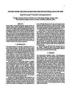
In indoor environments the most representative target of DATMO are people and other moving robots. The detection can be done by appearance-based approaches (using cameras) (Rosales and Sclaroff, 1999; Wang and Thorpe, 2002) or by feature-based approaches (using laser scanners) (Fod, et al., 2002; Schulz, et al., 2001, Kluge, et al., 2001). Both approaches rely on the prior knowledge of the targets. 3. SYSTEM ARCHITECTURE The DATMO system is LMS based and composed by three procedures: the data segmentation, the feature extraction, and the classification (see Fig. 1). This system receives LMS scan data and provides landmarks and classified objects, dynamically characterized in the workspace. All these procedures are properly presented in the next sections.

LMS Scan data

Segmentation Segments

Feature Extraction Feature Extraction Algorithm Primitive features

Classification Landmark dbase

Landmark detection

Pool

Features

Model dbase

Classification Reasoning

Objects Detected

Tracking

Landmarks

Objects Classified

Fig. 1. DATMO system architecture.

beam divergence. The constant C0 allows an adjustment of the algorithm to noise and strong overlapping of pulses in close range. The linear parameter C1 represents a lower bound associated with the LMS angular resolution (Dietmayer, et al., 2001). Segments have a minimum size established in the beginning (5 points) though pairs and isolated scan points are rejected. This is a very simple way of noise filtering. A local improvement could be done in each segment, testing near non-selected points to join the same object. 5. FEATURE EXTRACTION

4. SEGMENTATION In this work the LMS has a scan angle of 180°, with an angular resolution ∆α=0.5º. The laser range data measured in the instant k is represented by the set LMSK , of N data points Pi, with angle αi and distance value ri .   α  (1) LMS k =  Pi =  i  , i ∈ [ 0, N ]  ri    The segmentation represents scan points clusters that belong together. It is based in the computation of the distance between two consecutive scan points, calculated by

d ( Pi , Pi +1 ) = Pi +1 − Pi = ri 2+1 + r 2i −2ri +1ri cos ∆α

(2)

If the distance is less than the threshold chosen

d ( Pi , Pi +1 ) ≤ C0 + C1 min {ri , ri +1}

(3)

with

C1 = 2 (1 − cos ∆α )

After the segmentation process, the scanned segments found must be interpreted or recognized as features and objects. Features could be interpreted as primitive features, defined by geometric evidence (points, lines, circles and blobs), and high-level features generally referred to as landmarks (corners, columns, doors, etc.) (Arras and Siegwart, 1997). Primitive features are determined by an adaptation of the Hough transform (HT) (Hough, 1962), a line detection method. Several landmarks can be detected in indoor environments, being the traditional ones building static features, like those mentioned earlier, but some others, like wall angle deflections (convex and concave), static benches and dustbins, etc., can be detected as well. Due to the main objectives of this work and the characteristics of our real world environment, the following landmarks are considered: corners; convex and concave wall deflections, columns and static benches. 5.1. Hough Transform

(4)

the point Pi+1 belongs to the same segment as point Pi. The threshold is linear to the minimum distance between two consecutive scan points, due to the LMS

The HT (Duda and Hart, 1972) maps features in a sensorial space to sets of points in a parameter space, through the accumulation of evidence in a model space. It is very simple to use this technique with

laser range data because the transformation between the polar representation of the range data and the parametric spaces is straightforward. Line segments detection, HTL - The so-called normalparameterization (Duda and Hart, 1972) specifies a straight line by the angle θ of its normal and its algebraic distance ρ from the origin, see Fig.2a). From a set of data points {( x1 , y1 ) ,K, ( xn , yn )} we find a set of straight lines that fit them by transforming the points ( xi , yi ) into sinusoidal curves in the θ-ρ plane, expressed by the following transformation:

ρ = xi .cos θ + yi .sin θ

Associated to each line segment detected we propose the evaluation of the following ratio racc :

max(accumulated points) number data scan points

(x1,y1) ρ1 ρ3 ρ5

ρ4

θ2 ρ2 θ 1 x

a) NAP

(4)

Points belonging to the same line reproduce intercepting unitary curves, which accumulate their values in the accumulator interception points. Avoiding the representation of all unitary curves, an accumulator looks like Fig. 2b), with clusters of spikes, which represents line segments interpreted from the scan data. The highest spike inside a cluster is the line segment (ρi,θi) detected. Following the representation of the parametric data in the accumulator, we conclude that changes in the orientation of the real scan data produces significant changes in the accumulator location. As shown in Fig.2b, different line segments have different locations in the accumulator, and their mobility are represented by the arrows. After that, it is very simple to characterize a scan data segment in several line segments, with an algorithm that follows all data movements in the accumulator. New line segments are considered if there are more than three points accumulated in the new location. This algorithm is a straight forward procedure to characterize all the line segments included in a scan data segment without any other subsequent computation.

racc =

y

(5)

which can be interpreted as an accuracy measure, i.e. it represents the exactness of the LMS data inside its precision (≅1cm). If we have 20 data scan points and 20 points in the same accumulator cell, certainly the LMS acquired all the important points of a surface, and this line segment is a very good approximation of the real world. A line segment is defined as l = [ Pini , Pend , ρ ,θ , dim, racc ] , with points Pini and Pend, parametric values ρ and θ, dimension dim and ratio racc . All the lines associated to a data segment i are then defined as follows: Li = U  np j > 3 ∧ racc j > 0.5 ∧ dim j > 10cm , 0 < j < n lj

(6) Only the line segments with more than 3 points, more than half of the points correctly modelled, and dimension bigger than 10 cm are considered.

ρ1 ρ3 ρ4

ρ5

b)

180º

θ2

ρ2 0 0º

θ1

Fig. 2. a) The line normal-parameterization. Colinear points (xi,yi) can be parameterized by the parameters: θ - angle of the line normal, ρ - algebraic distance from the origin. In this example, point (x1,y1) is parameterized by (ρ1,θ1). b) Representation of the parametric accumulator (ρ,θ) showing the existing cells (ρi,θi) with Number of Accumulated Points – NAP bigger than 2, for the scan data segment represented in example 2a). The arrows show the sequential change in the accumulator location of parameterized point clusters, following a LMS scan made with an opposite clockwise direction.

Circle detection, HTC - Circles are parameterized in a three-parameters space (r,a,b) as follows:

r 2 = ( xi − a ) + ( yi − b ) 2

2

(7)

The triplet (r,a,b) will correspond to the accumulation cell where the largest number of cone surfaces intersect. For data circles with known radius r the search space can be reduced to 2D. If the radius is not known, the locus of points in parameter space will fall on the surface of a cone. Each point on the perimeter of a circle will produce a cone surface in parameter space. Real-time requirements - Considering the system specifications, some modifications to the HT method are done, to decrease the computational cost of extensive accumulators. Scan segment adaptive accumulators were developed to adapt the parameter space to the expected object class dimensions. The HT is applied to each segment when necessary, adapting the accumulators dimension to the segments constraints. For line detection, the HT is just applied inside a bounding box that covers all the segment scan data. The circle detection is performed in the Cartesian space. Considering just the segments that apply to be a circle, they have for sure three well defined points: the segment first, the segment nearest to the LMS, and the segment end. With these three points we formulate a convex surface that fits inside a circle, and calculate a geometric approximation for the circle centre. As shown in fig. 3, just a small gray area near the circle centre is parameterized, where the HT will be applied.

5.2. Feature Extraction Algorithm Features are detected from the work space geometric evidence by an adaptation of the HT. First we apply the HTL to all scan data segments, resulting a line segment characterization: position, orientation, dimension, and accumulator ratio. From these data, the angle between consecutive line segments belonging to the same scan data segment can be determined and a very simple reasoning is applied to characterize the segments with more than one linesegment, and lines with a very small racc, in circles or blobs. A brief description of the algorithm is shown in the next lines: IF (a line segment is unique in a scan segment data AND racc < 0.5) OR (a scan segment data have two non perpendicular line segments) OR (a scan segment data have more than two convex line segments) THEN apply HTC IF racc of the HTc > racc of the HTL THEN it is a circle ELSE it is a blob END ELSE it is a line segment END

Landmark detection needs the fusion of features data with tracking data and some heuristic rules. 6. CLASSIFICATION Object classification could be done by matching the primitive features with models of possible objects that could exist in the robot environment. Generally, most objects of interest in the robot’s or vehicle environment are either almost convex or can be decomposed into almost convex objects. A database of such possible objects is necessary, and a priori knowledge of the working environment is crucial to create it. In the beginning of this work only moving objects in indoor environments were in study. Meanwhile we realize that some landmarks are crucial to the modelling of the environment, and they can be used later in local navigation or SLAM tasks. We propose three different classes of objects, and a simple model for each one (see Fig. 4): Rectangular objects; Circle objects; and Human beings. Rectangular and circle objects are simple models, extracted from the HT accumulation of evidence in a model space. Human beings are modelled by compound models, extracted from two types of information: 1)- circle detection (geometric feature) and 2)-walking pattern (kinematic model). To characterize the object’s mobility we consider three different states: 0 – static object; 1 – dynamic object; X – undefined. An object is assigned as a static object when its dimensions are too big, scan segments bigger than dmax=150 cm, or when the tracking system perceives it as static.

.O

c

Pend

Pini Pnear

b a

Fig. 3. Based in scan points Pini and Pend, a geometric estimation for the circle centre is done, reducing the HTC accumulator to a small rectangular area (gray colour).

Or

r

Or

a)

Oc

b)

Op

c)

Fig. 4. Models extraction from the laser measurement system. a) model for a rectangular object; b) model for a circle object; c) model for a person.

Landmarks and immobilized mobile robots are examples of objects assigned as static object. Dynamic objects are assigned (‘1’) only by the tracking system. Although an object could be in an inactivity state, and at the beginning it was considered as static, once assigned dynamic it will be dynamic for ever. Undefined (‘X’) it is the first state assigned to an object with dimensions less than dmax, which need to be analysed. Small circles and blobs, are assigned ‘X’ during a small temporal window until the classification are concluded, because they can be human legs or any other object starting to be percepted. 6.1 People Modelling People modelling is under development, and it represents a distinct problem because it integrates two moving objects (legs) with an articulated movement, which depends on several variables, like the human leg length, the body velocity, etc. For simulation purposes we use a simplified model for walking (Alexander, 2001), which is presented in Fig. 5. First we need to remind ourselves what walking is like. One foot is set down just before the other is lifted. While a foot is on the ground, the knee of the same leg remains more or less straight. As we walk, our heads bob up and down. The centre of mass of the body is between, and a little above, the hip joints. Adapting this model to our case, it was assumed that the LMS is always positioned at the same height hLMS, and footprints of the walking movement (gray circles) are equal to a real scan data signature at height hLMS, in this case modelled by two circles with a distance dS (shoulders distance) between them, and radius of 10cm (considering a leg width of 20cm). The distance

vθ

vθ' θ

Vertical Plane

l

LMS Plane

hLMS wS 2lsinθ

Ground Level

Fig. 5. The walking model. In the vertical plane we have a kinematic sketch of the legs and body centre of gravity. On the ground level there are footprints for the time instants when the foot make contact with the ground (gray) and shadow footprints when the foot have no contact with the ground (dashed).

of a walking footstep is calculated by 2l sin θ , for a leg length l with angle θ.The velocity of the moving body is considered constant, vθ , despite its changes in the inclination. 6.2 Classification Algorithm After the feature extraction, the classification procedure separates landmarks from all other primitive features and possible objects, to reduce the list of possible objects to classify. Landmark detection – The procedure starts with a line segments analysis. The line segments with dimensions too large are considered static. After that, corners are identified and possible building geometric similarities that occur in junctions. In a typical LMS scan data set there is more information presented, which can not be determined just by angles, like corners not defined by two line segments, due to the LMS sensing position in the work space. In Fig. 6 there is a well defined corner (two perpendicular line segments) marked with a ‘ W ’ and another one that it is just the ending of a line (‘x’). This situation can be solved by testing building geometric similarities that occur in junctions. Starting on the corner landmarks ‘ W ’ we try to find other landmarks that exhibit the same geometric similarity. In Fig. 6 these landmarks are marked with ‘o’. Next, all circle primitive are analysed, to match columns and static benches. A static bench is represented in the same figure by two green circles with a rectangle between circle centers. All detected landmarks are registered in its proper database, and removed from the processing data. Object classification - An algorithm based on features data and some heuristic rules was developed to classify all the earlier enumerated classes of objects to be found in an indoor environment. With the knowledge of the number of line segments in each data segment, their dimensions and orientation, the most adequate model to match the segment being analysed can be select. The tracking system is crucial to match the objects position in the current scan with the later estimated positions.

a)

b)

Fig. 6. a) LMS data points in black and red; b) Line segments are marked in blue and landmarks signalized by: x – undefined ends for line segments; o – real geometric similarity; W – real corner. A static bench is represented in green.

Tracking - The tracking system is Kalman filter based, estimating the position and velocity of an object's point that could be easily identifiable in successive scans and appropriately represents the object's movement. This point for each object is its model centre. To perform this estimation a kinematic model of the object (white noise acceleration model following Kohler (1997)) is used. The motion is considered to be the superposition of the ideal basic motion with constant velocity and white noise. The white noise illustrates the acceleration that is time varying. Separated Kalman filters are applied independently to the x and y coordinates, to speed the calculus. 7. EXPERIMENTAL TEST The proposed DATMO system has been implemented in a mobile robot and tested extensively in simulation runs using MATLAB™. Real tests were done using the Player software tools (Gerkey, et al., 2003), a robot device server, to control a Pioneer 2DX and the Sick LMS200. The LMS perceptual range was set to 8m, at a rate of 5 Hz. A real experiment is presented with the robot tracking two persons walking along a building hall. One of them is pulling a mobile platform with a wire at a constant distance (≅2m). The building hall has several well defined landmarks, like two columns and two static benches (see a panoramic view of the experimental environment shown in figure 7a). The trajectory of the person pulling the mobile platform has two phases, the first one is easy to follow by the DATMO system, the second one is behind the columns, with occlusion stages for the person and for the mobile platform (see Fig.7b). In Fig. 7c) shows a picture of our interface developed in OpenGL, with the landmarks represented in red (columns) and redyellow (static benches), the mobile platform is represented by red circles, person footsteps are represented by black circles, scan data with blue at the floor level and scan segments with cyan at the LMS level.

9. ACKNOWLEDGEMENTS

a)

This work was partially supported by a PhD student grant (BD/1104/2000) given to the author Daniel Castro by FCT (Fundação para a Ciência e Tecnologia). The author Urbano Nunes acknowledges the support given by FCT (POSI/SRI/33594/2000). We thank to João Xavier and Marco Pacheco for their contribution in the real test. REFERENCES

b)

c) Fig. 10. Real test with the Pioneer robot aligned with the wall, in a building hall. a) Panoramic view of the experiment scene. b) Snapshots of the experiment, two persons are walking along the hall, one of them is pulling a mobile platform. c) Picture of an OpenGL interface with all the experiment represented. Landmarks are detected and moving objects are tracked.

There are some errors of the classification system in this picture, like the red circles near the corner and near the benches, which will be removed in the future. 8. CONCLUSIONS The proposed algorithms demonstrate some robustness in real time applications, for detection, classification and tracking of multiple moving obstacles in indoor environments. The people modelling development is not already concluded. Future work must cover occlusion and dataassociation problems. Performance indexes must be evaluated for the DATMO system, covering different object classes, object velocities, and occlusion situations.

Alexander R. (2001). Modelling, step by step. +Plus, 13. (http://plus.maths.org/). Arras K. and R.Siegwart (1997). Feature-Extraction and Scene Interpretation for Map-Based Navigation and Map-Building. In Proc. of SPIE, Mobile Robotics XII, Vol. 3210. Bar-Shalom Y. and X.-R. Li (1995). Multitarget-Multisensor Tracking: Principles and Techniques. YBS, Danvers, MA. Castro D., U. Nunes and A. Ruano (2002a). Obstacle Avoidance in Local Navigation. In IEEE Mediterranean Conference on Control and Automation MED 2002, Lisbon. Castro D., U. Nunes and A. Ruano (2002b). Reactive Local Navigation. In IEEE Int. Conference on Electronic and Industrial IECON 2002, pp.2427-2432, Sevilla. Dietmayer K., J. Sparbert and D. Streller (2001). Model Based Object Classification and Tracking in Traffic Scenes from Range Images. In IEEE Intelligent Vehicle Symposium IV2001, , paper 2-1, May, Tokyo. Duda R.O. and P.E. Hart (1972). Use of the Hough Transformation to Detect Lines and Curves in Pictures. Communications of the Association of Computing Machinery, 15(1), pp.11-15. Fiorini P. and Z. Shiller (1998). Motion Planning in Dynamic Environments using Velocity Obstacles. Int. Journal on Robotics Research, 17(7), pp.711-727. Fod A., A. Howard and M. J. Mataric (2002). A Laser-Based People Tracker. In IEEE Int. Conference on Robotics and Automation ICRA’02, pp.3024-3029, Washington. Fuerstenberg K. and V. Willhoeft (2001). Object Tracking and Classification using Laserscanners – Pedestrian Recognition in urban environment. In IEEE Intelligent Transportation Systems Conference, pp. 453-455, Oakland (CA), USA. Fox D., W. Burgard. and S. Thrun (1997). The Dynamic Window Approach to Collision Avoidance. IEEE Robotics and Automation Magazine, 4(1), pp. 23-33. Gerkey B.P., R.T. Vaughan and A. Howard (2003). The Player/Stage Project. http://playerstage.sf.net . Hough P.V.C. (1962). Method and Means for Recognizing Complex Patterns. US Patent 3.069.654, Dec. 18. Kluge B., C. Köhler and E.Prassler (2001). Fast and Robust Tracking of Multiple Moving Objects with a Laser Range Finder. In IEEE Int. Conference on Robotics and Automation ICRA’01, pp.1683-1688, Seoul. Kohler M.(1997). Using the Kalman Filter to Track Human Interactive Motion - Modelling and Initialization of the Kalman Filter for Translational Motion. Technical Report 629, Informatik VII, University of Dortmund. Latombe J-C. (1991). Robot Motion Planning. Kluwer Academic Publishers, Boston. Mendes A., L. Conde and U. Nunes (2004). Multi-Target Detection and Tracking with a Laserscanner. In IEEE Intelligent Vehicles Symposium IV04, June, Parma. Rosales R. and S. Sclaroff (1999). 3D Trajectory Recovery for Tracking Multiple Objects and Trajectory Guided Recognition of Actions. In IEEE Int. Conference on Computer Vision and pattern Recognition, pp. 123, June. Shiller Z., F. Large and S. Sekhavat (2001). Motion Planning in Dynamic Environments: Obstacle Moving Along Arbitrary Trajectories. In IEEE Int. Conference on Robotics and Automation ICRA’01, pp.3716-3721, Seul. Schulz D., W. Burgard, D.Fox and A.Cremers (2001). Tracking Multiple Moving Targets with a Mobile Robot using Particle Filters and Statistical Data Association. In IEEE Int. Conference on Robotics and Automation ICRA’01, pp.16651670, Seul. Wang C-C and C. Thorpe (2002). Simultaneous Localization and Mapping with Detection and Tracking of Moving Objects. In IEEE Int. Conference on Robotics and Automation ICRA’02, pp.2918-2924, Washington.