1994
IEEE TRANSACTIONS ON AUDIO, SPEECH, AND LANGUAGE PROCESSING, VOL. 14, NO. 6, NOVEMBER 2006
Feature Extraction for the Prediction of Multichannel Spatial Audio Fidelity Sunish George, Student Member, IEEE, Slawomir Zielinski, and Francis Rumsey
Abstract—This paper seeks to present an algorithm for the prediction of frontal spatial fidelity and surround spatial fidelity of multichannel audio, which are two attributes of the subjective parameter called basic audio quality. A number of features chosen to represent spectral and spatial changes were extracted from a set of recordings and used in a regression model as independent variables for the prediction of spatial fidelities. The calibration of the model was done by ridge regression using a database of scores obtained from a series of formal listening tests. The statistically significant features based on interaural cross correlation and spectral features found from an initial model were employed to build a simplified model and these selected features were validated. The results obtained from the validation experiment were highly correlated with the listening test scores and had a low standard error comparable to that encountered in typical listening tests. The applicability of the developed algorithm is limited to predicting the basic audio quality of low-pass filtered and down-mixed recordings (as obtained in listening tests based on a multistimulus test paradigm with reference and two anchors: a 3.5-kHz low-pass filtered signal and a mono signal). Index Terms—Frontal spatial fidelity, ridge regression, spatial feature, spectral feature, surround spatial fidelity.
I. INTRODUCTION
T
HE PAST ten years have seen the extension of multichannel audio from theatres to home cinema [1]. Also TV/radio broadcast and audio/video on-demand services in multichannel audio have become more popular. Several companies have introduced wide and varied services and products to satisfy the needs of customers. The development phase of all of these products or services normally has to pass through listening tests in order to evaluate the quality of the reproduced audio. However, such listening tests are time consuming and expensive. So-called objective methods involving physical measurement are an alternative solution in certain circumstances to overcome these difficulties. However, current objective methods have limitations such that they cannot entirely replace listening tests. Research leading towards the objective prediction of sound quality has been undertaken since 1979 [2]. Since then, a number of advancements and novel methods have been proposed as reported in [3]–[8] and [9]. In 1998, ITU’s attempt to codify a standard for the objective evaluation of audio quality Manuscript received February 1, 2006; revised July 17, 2006. The associate editor coordinating the review of this manuscript and approving it for publication was Dr. Peter Kroon. The authors are with the Institute of Sound Recording, University of Surrey, Guildford, Surrey, GU2 7XH, U.K. (e-mail:
[email protected].;
[email protected];
[email protected]). Digital Object Identifier 10.1109/TASL.2006.883248
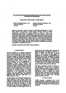
resulted in a standard (ITU-R BS.1387) [10], known as Perceptual Evaluation of Audio Quality (PEAQ) [11]. In recent years, several improvements have been proposed to PEAQ such as [12]–[16] and [17]. However, none of them except [16] addressed issues relating to the evaluation of multichannel audio quality. In [16], Torres et al. converted 5.1-channel recordings to a binaural format using head-related transfer functions (HRTFs), and the basic version of the PEAQ model was used for quality prediction. The use of such a binaural “front end” to PEAQ does not overcome the basic problem that PEAQ takes no account of spatial quality changes in stereo or multichannel recordings. Hence, this method is insufficient for multichannel audio quality prediction. As mentioned previously, multichannel audio (especially 5.1 surround audio) has become particularly prevalent in commercial systems and applications and hence an objective method for the evaluation of multichannel audio quality has great importance. In [37], Karjalainen describes a number of features that might be used for the prediction of multichannel audio quality. However, there has been no work reported so far, in the context described here, that uses them for the prediction of multichannel audio quality. In [18], an algorithm to evaluate multichannel audio quality is proposed. However, its prediction capability is limited to some specific degradation types only (bandwidth limitation). The algorithm proposed in this paper is the first step towards a comprehensive algorithm to predict multichannel audio quality. Letowski describes the two attributes of sound quality as timbral quality and spatial quality [19]. Also, ITU has proposed two subattributes of basic audio quality as “Front image quality” and “Impression of surround quality” for multichannel audio with more than two audio channels [20], which can be considered as two attributes of so-called sound quality as proposed by Letowski. Later in [21], Rumsey et al. demonstrated the relative importance of spatial and timbral fidelities. They showed that two attributes, frontal spatial fidelity and surround spatial fidelity, were statistically significant and, therefore, important for the prediction of the basic audio quality. The aim of this paper is not to propose an algorithm to replace the existing PEAQ model with an equivalent “multichannel PEAQ” algorithm, but to describe a number of features that can be extracted from multichannel audio recordings to represent the spatial audio quality attributes—frontal spatial fidelity and surround spatial fidelity. Frontal spatial fidelity can be defined as the global attribute that describes any and all detected differences in the “spatial impression” inside the frontal arc (see nonshaded area in Fig. 1) of the multichannel audio setup, between the reference and the evaluated recording. The definition of the surround spatial fidelity can be given as the
1558-7916/$20.00 © 2006 IEEE
GEORGE et al.: FEATURE EXTRACTION FOR THE PREDICTION OF MULTICHANNEL SPATIAL AUDIO FIDELITY
1995
TABLE I DEGRADATIONS WITH BANDWIDTH LIMITATION (FOR CALIBRATION EXPERIMENT)
TABLE II DOWN-MIXED VERSIONS (FOR CALIBRATION EXPERIMENT) Fig. 1. Multichannel audio setup: Frontal arc and the angle outside frontal arc.
global attribute that describes any and all detected differences in the spatial impression outside the frontal arc (see shaded area in Fig. 1) of the multichannel audio setup, between the reference and the evaluated recording. The design of a predictor involves two phases—calibration and validation. Calibration is the fundamental process used to achieve consistency of prediction using a set of variables and a desired output. The validation phase verifies the accuracy of the calibration with a new set of test cases. It is important to emphasize here that the developed algorithm was calibrated using the database obtained from the listening tests conforming to the modified ITU-R BS.1534 (MUSHRA) Recommendation [20] with a mono signal used as an additional anchor. Consequently, the applicability of the developed predictor is limited to the scores obtained in the context of MUSHRA conformant listening tests with a mono signal used as one of the supplementary anchors (this issue will be discussed in more detail in Sections II and VII). This paper is arranged as follows. In Section II, a brief description of the database used for the calibration is presented. Section III is dedicated to illustrating the various features extracted from the recordings for the models, and Section IV describes how a subset of features has been derived. Section V speaks about the optimization process that is used for the calibration of the model and the results of calibration. The details of a validation experiment are offered in Section VI. The results of calibration and validation are discussed in Section VII. The paper ends with conclusions and suggestions for future work in Section VIII. II. SUMMARY OF CALIBRATION DATABASE The database used for the calibration was obtained from a series of listening tests conducted in an ITU-R BS.1116-compliant listening room at University of Surrey, U.K. The strategy used in the listening tests was a modified ITU-R BS. 1534 Recommendation as described in [22]. A summary of the experiment is given in the following paragraphs and a more detailed description can be found in [22]. Twelve program items were used for the listening tests, selected from movies, music recordings, TV programs, etc.
Two types of program items were used in the calibration database—these being recordings with “F-B” and “F-F” audio scene characteristics. An audio scene with “F-F” characteristics means that the front and rear channels contained clearly distinguishable audio sources. The listening impression is similar to that when a listener is surrounded by a group of instruments in an orchestra. The listening impression from a recording with the “F-B” characteristic is similar to that experienced in a concert hall. That is, the front channels contain clearly perceived audio sources and the rear channels contain mainly reverberant sounds and room response. A detailed description of these characteristics can be found in [23] and [24]. The program items were processed so as to have two types of quality degradation (see Tables I and II), by means of bandwidth limitation and down-mixing. For down-mixing, the algorithms presented in [36] were used. From Table II, it can be seen that all the down-mixed versions (except the 1/2 down-mixed recordings) do not have surround channels after the down-mixing. One may question how the surround spatial fidelity of such recordings can be evaluated when no surround channels are present (i.e., when the contents of the recordings are down-mixed to 3, 2, and 1 channels in the front). However, some past experiments have shown that even for mono or two-channel stereo reproduction modes listeners still perceived some sort of surrounding spatial impression or envelopment, and hence they graded surround spatial fidelity for these recordings at a higher level than expected [22]. It was hypothesized that this phenomenon could be attributed either to interactions between the loudspeaker signals and the room reflections or to the signal interactions caused by the front loudspeakers at the ears of the listener. The detailed examination of this phenomenon, however, is beyond the scope of this study. Bandwidth limitation was applied to the recordings by following two different approaches. In the first approach, all the channels present in the recordings were processed with filters
1996
IEEE TRANSACTIONS ON AUDIO, SPEECH, AND LANGUAGE PROCESSING, VOL. 14, NO. 6, NOVEMBER 2006
III. FEATURES EXTRACTED FOR THE PREDICTION A number of features were extracted from the recordings to check their suitability for predicting the subjective grades. As mentioned in the previous section, the degradations applied to the recordings were created by bandwidth limitation and downmixing. Therefore, the primary aim in the study reported here was to find some features that could represent the difference between the spectral and spatial characteristics of the reference and test recording. Hence, the features extracted could be divided mainly into two categories—spectral features and spatial features—on the basis of the characteristics that they carried. All the computations described in this section were carried out using Matlab 7.0 in a Mac OSX 10.3.9 environment. A. Spectral Features Fig. 2. Grading scale used for the listening tests.
having equal cutoff frequencies. In the second approach, the channels were processed with filters differing in cutoff frequencies. In total there were 138 recordings. Reference recordings selected from the various sources were used in the listening test with 48-kHz sampling frequency at 16-bit resolution. The calibration database was obtained in listening tests designed according to a modified ITU-R BS.1534 (MUSHRA) Recommendation [20]. The main modification was that instead of asking the listeners to assess the basic audio quality, they were asked to grade two other attributes independently, namely frontal spatial fidelity and surround spatial fidelity. Each subject was asked to grade frontal spatial fidelity and surround spatial fidelity of the test recording by comparing the corresponding item to the reference recording. A 100-point scale as shown in Fig. 2 was used for the grading. The MUSHRA test is a multistimulus test in which two mandatory signals have to be included in the pool of items to be graded: the hidden reference (original recording) and a 3.5-kHz low-pass filtered version of the original recording (so called anchor). According to the ITU-R BS.1534 recommendation, “other types of anchors showing similar types of impairments as the system under test can be used” [20]. Hence, an additional mono anchor was also used in the listening tests. In line with the recommendation, the listeners were instructed to assign the top value from the scale (100) for the hidden reference. In other words, regardless of the absolute perceptual magnitude of the frontal spatial fidelity or surround spatial fidelity, the listeners were instructed to assess the unprocessed original recording as 100. Although the listeners were not given any specific instructions as to how they should assess the spatial fidelity of the anchors, a visual inspection of the database obtained in the listening tests revealed that for the mono anchor the participants gave scores spanning only the bottom range of the scale. Consequently, in order to mimic the way in which the subjects assessed the stimuli normalization of the objective features was necessary (see Sections III-A2 and III-A3). As a result, the applicability of the algorithm described in this paper is limited to the prediction of scores obtained using the listening tests similar in their design to the one described previously.
To extract the spectral features, the surround recordings were down-mixed to a mono recording by summing all the individual channels. This mono recording was then processed in different ways to build the features as described in the following paragraphs. Spectral centroid and spectral rolloff: The center of gravity of the magnitude spectrum of the short-time Fourier transform (STFT) of an audio signal is termed the spectral centroid [25]. Spectral centroid is a measure of spectral shape and is the objective representation of the subjective attribute “brightness” [42]. For the computation of spectral centroid and spectral rolloff (see below), the down-mixed mono signal is divided into frames of size 42.67 ms and the Fourier transform is performed on each frame. The centroid and rolloff would vary from recording to recording depending on the type of music and recording. By computing the difference feature (as described in Section III-A2), the perceptual difference between the reference and test recording can be modeled. The spectral centroid is defined as the average frequency weighted by magnitudes divided by the sum of the magnitudes. The basic calculation of this feature is given as
(1)
where is the magnitude of the Fourier transform of the frame and frequency index . Similarly, in the basic calculation of spectral rolloff, the determines where the 95% of the frame’s magnitude point is defined as the smallest value of is achieved [26]. Thus, such that the inequality (2) is satisfied. Formulas (1) and (2) were applied to each frame of the test and reference down-mixed recordings. A set of features were derived as described in Sections III-A1–A3. 1) Averaged Basic Feature Across the Frames: The average value of the basic features across all frames was calculated for
GEORGE et al.: FEATURE EXTRACTION FOR THE PREDICTION OF MULTICHANNEL SPATIAL AUDIO FIDELITY
1997
the reference and test recordings. The averaged feature is defined as
(3) where is the frame number, is the basic feature (either spectral centroid or spectral rolloff) calculated for frame , and represents the total number of frames in the audio excerpt. 2) Difference Feature: According to the ITU-R BS. 1534 Recommendation, listeners are expected to evaluate the perceptual differences between the reference and the test recordings [20]. As a result, the scores obtained in the listening tests retain only information about the perceptual differences between the reference and the test items, not the absolute magnitude of the graded attribute. Consequently, in order to mimic the way the listeners evaluated spatial audio fidelity, there was a need to introduce some form of normalization of scores in the algorithm for the purpose of automatic prediction of the listening test scores. For example, the difference feature was introduced to represent the perceptual difference between the reference and test recording. This feature was defined as
Fig. 3. Coherence spectrum obtained for a reference recording and a test recording degraded by Hybrid C process.
(4)
(8)
where and are the averaged spectral centroid or spectral rolloff calculated for the reference and test recording. Throughout this paper, the subscripts and correspond to reference and test recordings, respectively. 3) Rescaled Feature: Visual inspection of scores obtained for spatial fidelities in the listening tests revealed that for a given original recording and its processed versions the scores spanned almost the whole grading scale regardless of the actual magnitude of perceptual differences between the reference and test recordings (the reference recordings were always graded using the top value of the scale whereas the mono and 3.5-kHz anchors were typically graded using the bottom range of the scale). This phenomenon is well known in psychology and is referred to as range equalization bias [43]. In order to mimic this phenomenon, it was decided to rescale the features so that for a given original recording and its processed versions the features spanned the range of values from a fixed maximum value (for reference) to a fixed minimum value (for anchor). Hence, the spectral features were rescaled to a range between 100 and 20. The rescaled spectral feature was generated by rescaling the averaged basic feature in the following way:
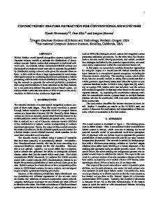
was the coherence estimate between the reference where and were the power specand test recording; was the tral densities of reference and test recordings; cross power density of reference and test recording. , , and were obtained from the mono versions of reference and test recordings. For the computation of this feature, the built-in function “mscohere“ from Matlab 7.0 was used [27]. An example of the coherence spectrum calculated between the mono signals obtained from a reference and test recording limited in bandwidth by Hybrid C strategy is given in Fig. 3. The mono signals of test recordings were made using a time-alignment algorithm in order to compensate for the group delays caused by low-pass filters. The value of coherence was near to unity at those frequencies where the signal had not been affected by the low pass filtering. In the “Hybrid C” condition, different channels were filtered using filters with different cutoff frequencies (18.25 kHz for front left and right, 3.5 kHz for center and 10 kHz for surround channels). As seen in the example for Hybrid C, the filtering did not affect any channels up to 3.5 kHz of the spectra and, hence, the coherence was near to unity until that frequency. From the coherence spectrum, the center of gravity of the spectrum (COH) was computed by applying (1) and by replacing the magnitudes M by coherence values.
(5) where and expressions:
were calculated as given in the following
4) Spectral Coherence Based Feature: A coherence spectrum is obtained by computing the correlation between the corresponding frequency indices of various frames present in the reference and test recordings. It is calculated using the following expression:
B. Spatial Features (6) (7) where and are the basic spectral features computed for a hidden reference and 3.5-kHz anchor, respectively.
The purpose of the spatial features was to represent the perceptual difference between the spatial characteristics of the reference and the test recording. The spatial features presented here can be categorized into two types: 1) interaural cross correlation (IACC)-based features and 2) energy-based features. For computing the IACC-based spatial features, the multichannel audio
1998
IEEE TRANSACTIONS ON AUDIO, SPEECH, AND LANGUAGE PROCESSING, VOL. 14, NO. 6, NOVEMBER 2006
recordings were converted into a binaural form using convolution of loudspeaker signals with head related transfer functions (HRTFs) corresponding to the angles at which respective loudspeakers were positioned (see Fig. 1). For the purpose of this study, the database of HRTFs measured by Gardner and Martin [28] was adopted. The energy-based features were basically the ratio of energies of the loudspeaker signals computed in different ways as described in Sections III-B4 and III-B5. 1) Broadband IACC: Interaural cross correlation coefficient (IACC) is an objective measure used in concert hall acoustics. It is calculated from the head related impulse responses obtained from a dummy head placed inside a concert hall. It is computed by the following expression [38]: (9)
where and represent the left and right channels of binaural recording and argument is in the range of 1 ms. The basic computation of IACC was done using (9). The IACC measured with music signals has different properties compared to that obtained from impulse responses. The measurement based on music signals depends on the average length of notes, the presence of vibrato, and also other factors like the direct-to-reverberant energy ratio. Measuring IACC with music has a basis in perception as it is related to the way humans perceive IACC during a concert [39], [40]. IACC is a useful physical correlate of source spaciousness or the subjective phenomenon of apparent source width [29]. In this study, the broadband IACC was calculated for each 42.67-ms frames on the corresponding binaural version of reference and test recordings. The cross correlation IACC between left and right channels of the binaural signal was computed for the argument ranging from 1 to 1 ms and the maximum value was chosen. Since the cross correlation varied widely from frame to frame, it was decided to create the feature for the prediction by averaging the maxima of IACC values in all the frames present in a recording. This averaging resulted in a better representation of IACC for the graded excerpt. 2) Rescaled Broadband IACC: As mentioned previously, in order to mimic the way the listeners evaluated spatial audio fidelities, there was a need to introduce some form of normalization of scores in the algorithm for the purpose of automatic prediction of listening test scores. Therefore, the IACC-based feature described in Section III-B1 was rescaled to the range between 1 and 0 by applying the (10) which is a simplified form and were subof (5). This equation was obtained after stituted by the IACCs obtained for hidden reference and mono anchor in (6) and (7). The (10) was obtained after substituting since for a mono recording, IACC would be equal to 1
as shown in Fig. 1. In the second case, the head was rotated 90 clock-wise. 3) Rescaled Low-Frequency Band IACCs: The calculation of rescaled low-frequency IACCs was done in a way similar to that mentioned in Section III-B2 above except that it was computed for three octave filter bands with center frequencies of 500, 1000, and 2000 Hz. The rescaling of the IACC was done as described in Section III-A3. A feature was formed by choosing the maxima of the three IACCs from the three bands. The rescaled IACC features were then calculated for seven dummy head rotations of 0 , 30 , 60 , 90 , 120 , 150 , and 180 . 4) Back-to-Front Energy Ratio: Morimoto describes a relationship between the spatial impression and the loudspeaker energy in a multichannel audio setup [30]. Back-to-front energy ratio was selected as a feature since it was a descriptor of the energy distribution in a multichannel audio soundfield and it had a significant effect on the spatial impression provided to the listeners. The decision to use back-to-front energy ratio instead of front-to-back one was to avoid a possibility of division by zero if there was a zero energy in the rear channels (as described earlier in Table II, some down-mixed recordings do not have any signals in the rear channels). The back-to-front energy ratio is defined as follows: (11) represents the sum of the rms levels of the signals in where represents the sum of the rms levels front speakers, whereas of the signals reproduced by the rear channels. , another feature, In addition to back-to-front ratio called , was included in the algorithm. This new feature was calculated using the same equation as before; however, and were replaced with average rms levels in the front and rear speakers, respectively. 5) Lateral Energy (LE): In concert hall acoustics, lateral is considered to be an objective measurement of lisgain tener envelopment [31]. Since listener envelopment is directly related to the sense of spatial impression, it was decided to check whether this feature could be used as a predictor of the frontal spatial fidelity or the surround spatial fidelity. The lateral gain can be computed as follows: (12) is the energy of a concert hall impulse response meawhere is the energy sured through a figure-of-eight microphone and of an impulse response measured through an omnidirectional microphone. The figure-of-eight microphone and the omnidirectional microphone are modeled using the following equation: (13)
(10) where and are broadband IACC calculated for reference and test recordings, respectively. This feature was calculated for head positions of 0 and 90 . In the first case (0 ) the head was facing the center loudspeaker,
where represents the angle of sound incidence and is a cofor an efficient depending on the type of a microphone ( omnidirectional and for a figure-of-eight microphone). There were two main problems making a direct implementation of (12) impossible in the study. First, in contrast to concert hall acoustics where almost all measurements are undertaken
GEORGE et al.: FEATURE EXTRACTION FOR THE PREDICTION OF MULTICHANNEL SPATIAL AUDIO FIDELITY
using the impulse responses, in the current study only the final recordings were available (e.g., musical signals) without access to any impulse responses of the recording studios or recording equipment. Therefore, it was necessary to use continuous signals instead of impulse responses in order to calculate (13). Second, the numerator in (12) was originally intended to measure the energy of late lateral reflections (hence 80 ms used as a lower integration limit [31]). In the current study, the measurement of late lateral reflections was not very important as many of the recordings employed in the listening tests contained predominantly direct audio sources panned around a listener. Hence, the original value of 80 ms used as a lower integration limit in the numerator was replaced by 0. Due to the significant modifications described above, it was decided to refer to this modified feature as a “lateral energy” (LE) as it better reflected the current authors’ intentions in which this parameter was used. The lateral energy (LE) was computed from the loudspeaker signals, and the values were selected as the corresponding speaker azimuths of the multichannel audio setup used in the listening tests (0 , 30 , 110 , 330 , and 250 ). The upper limit of in (12) was impractical to implement and, hence, the integration time was set to the duration of the recordings. It was decided to calculate three separate features based on ) was obtained using the diLE. The first feature (called rect calculation of LE, whereas the second feature was estimated as the difference between the LE for reference and test record. The third feature was computed using the ings rescaling strategy presented in Section III-A3 by substituting the as the values obtained for mono anchor. value for The usefulness of this new lateral energy-based feature is questionable. Informal predictions using the LE-based features independently in a linear regression model showed that they were not very important for the prediction of frontal and surround spatial fidelities. In addition to the features described in the previous paragraphs, selected interactions were also examined between LE, , and all other direct features. Interactions were examined by calculating products of selected features and using them in the model. The purpose of energy-based spatial features was to represent listener envelopment and, hence, the authors believed that these features could significantly interact with the other features even if they failed to be useful predictors on their own. The final list of extracted features is presented in Table III. For clarity, the table does not include any interactions between features. IV. SELECTION OF THE EXTRACTED FEATURES As described in the previous section, a number of features were extracted from the recordings and used for the prediction of frontal spatial fidelity and surround spatial fidelity. The details of all direct features used in the regression model are presented in Table III. As described previously, two sets of interaction features were built by multiplying the selected direct and lateral energy features with back-to front-ratio and used in the regression model. Some of the features extracted have similar characteristics because they attempt to represent the same properties. Consequently, the results showed that many of the features (partic-
1999
TABLE III LIST OF EXTRACTED FEATURES
ularly IACC-based features at different head positions) were highly correlated. If these features had been used directly in a multiple linear regression model the results would, therefore, have been biased by multicolinearity, resulting in an abnormal variance inflation factor (VIF) [32]. There are many regression analysis techniques that are robust to multicolinearity, such as partial least squares regression, principal component regression, ridge regression, etc. These methods tend to yield the same or similar results. For this study, ridge regression [33] was chosen as an alternative method to multiple linear regression. In ridge regression, a shrinkage value needs to be specified. Ridge regression shrinks the regression coefficients by imposing a penalty on their size [41]. Selection of a shrinkage value ( ) for ridge regression is a tradeoff between the biased coefficients and the magnitude of standard error of estimate (SE). If the shrinkage value is chosen to be very small, the model has high correlation and low standard error, but the coefficients are biased. This situation is very similar to that of a multiple linear regression and, thus, the model normally would not pass a validation test. Hence, the selection of the shrinkage value was done as a compromise to minimize the standard error of estimate and biasing so as to obtain a stable model [33], [34]. The calibration of the models for frontal spatial fidelity and surround spa. The macro tial fidelity was done with shrinkage value “RIDGEREG“ available with the SPSS [35] was used to predict the spatial fidelities. A. Features for Frontal Spatial Fidelity Prediction First, the prediction of frontal spatial fidelity was done. The frontal spatial fidelity was the dependent variable and the extracted features were the independent variables. The correlation and the standard error (SE) were calculated for the prediction. These were then related to the original scale used for the evaluation of frontal spatial fidelity (a 100-point scale as shown in Fig. 2). All the standard errors mentioned throughout this paper are relative to this scale. The initial model showed a high correlation with a low standard error . However, after the analysis of the model it was found that not
2000
IEEE TRANSACTIONS ON AUDIO, SPEECH, AND LANGUAGE PROCESSING, VOL. 14, NO. 6, NOVEMBER 2006
TABLE IV FRONTAL SPATIAL FIDELITY (SELECTED FEATURES AFTER THE FIRST ITERATION)
TABLE V FRONTAL SPATIAL FIDELITY (MODEL AFTER FINAL ITERATION)
TABLE VI SURROUND SPATIAL FIDELITY (SELECTED FEATURES AFTER THE FIRST ITERATION)
Fig. 4. Selected features from the first iteration of the frontal spatial fidelity prediction.
all of the features were important for the prediction. Hence, the decision was made to retain only those features that exhibited relatively high importance in the prediction. Table IV shows the unstandardized coefficients , standardized coefficients (Beta), -values, and 95% confidence intervals of these features obtained from the initial model. The values are also known as regression coefficients and are used in the regression equation to do the prediction. The Beta values of each feature describe how well it fits in a regression model and how important it is compared to other features. The higher the magnitude of Beta values, the greater the importance of a feature in a regression model. Fig. 4 shows the Beta values of important features with its 95% confidence intervals. The selection of the features was done by following an iterative process in order to obtain a simplified model. The more features present in a regression model, the greater the cost of computation and model maintenance. The process of finding a suitable model is a compromise between the number of features and error variance. The number of iterations may vary depending on the number of features used for the prediction and the criteria used for selecting the important features and, hence, several iterations may be required to produce an adequate model [33]. In the first step of the iteration, those features with relatively small standardized coefficients were removed. The important features obtained after the first iteration are given in Table IV. Surprisingly, showed high Beta value in the first iteration. In the second iteration, important features found from the first iteration were applied to the regression model. It was found that
the feature , , and showed a relatively low Beta value compared to that of others. The low Beta value of in the second iteration indicated that it was not a useful feature as anticipated in the previous section. Therefore, they were removed from the model and the remaining features were applied to a regression model (third iteration). Throughout this process, the retained features were monitored to determine whether they were statistically significant or not. The resulting model obtained after the third iteration is given in Table V. Only the , COH, , following features were retained in the model: , , and (the interaction between the and broadband IACC measured at 90 head azimuth). Almost all of the interaction features except were found to be unimportant. The selected feature set for the prediction of frontal spatial fidelity was statistically significant at . Table V shows the result from the final iteration. The high values of Beta, 95% confidence intervals of same sign and high magnitudes of -values in Table V support the fact that the selected features in the model were important and statistically significant at level. B. Features For Surround Spatial Fidelity The simplified subset of features for the prediction of surround spatial fidelity was selected using a similar procedure to that described in the previous subsection. The first iteration resulted in the selected features listed in Table VI. The model showed a correlation of 0.96 with a standard error of 9.09. Fig. 5 shows the Beta values of important features with associated 95% confidence intervals. In the final iteration, it was found that the relevant features chosen from the previous iteration were statistically significant at and important for the prediction of surround spatial
GEORGE et al.: FEATURE EXTRACTION FOR THE PREDICTION OF MULTICHANNEL SPATIAL AUDIO FIDELITY
2001
TABLE VII SURROUND SPATIAL FIDELITY (MODEL AFTER FINAL ITERATION)
Fig. 5. Selected features from the first iteration of the surround spatial fidelity prediction.
Fig. 7. Scatter plot of the surround spatial fidelity prediction.
B. Calibration Model for Surround Spatial Fidelity Fig. 6. Scatter plot of the frontal spatial fidelity prediction.
fidelity. The high values of Beta, 95% confidence intervals with same sign and high magnitudes of -values tell that the selected features were important and statistically significant. Section V presents the prediction of the two spatial fidelities using the subsets of features obtained from the iterative process described previously. V. RESULTS OF MODEL CALIBRATION A. Calibration Model for Frontal Spatial Fidelity Table V discussed above shows a list of all the important features retained in the regression model predicting frontal spatial fidelity. An equation was built using values in Table V and frontal spatial fidelity was predicted. The predicted results with a standard error of 9.33. showed a correlation of The graph given in Fig. 6 shows a scatter plot of the prediction.
The calibration procedure followed for the prediction of surround spatial fidelity was similar to that of frontal spatial fidelity. The surround spatial fidelity was predicted using the revalues given in Table VII. The gression equation built by with a standard error model showed a high correlation of estimate 8.87. The scatter plot of surround spatial fidelity prediction is shown in Fig. 7. VI. VALIDATION EXPERIMENT The validity of the model described previously had to be checked in order to verify whether it could be generalized. Therefore, another listening test was conducted with a new set of audio recordings and listeners. In order to reduce the possibility of bias, the validation experiment was conducted by a person who was not involved in the experiments that resulted in the creation of the calibration database. According to [24], multichannel audio recordings exhibiting “F-F” characteristic are “critical” program materials for revealing perceptual changes in audio quality caused by downmixing. Therefore, the validation experiment consisted of recordings with “F-F” audio characteristic only. However, it is
2002
IEEE TRANSACTIONS ON AUDIO, SPEECH, AND LANGUAGE PROCESSING, VOL. 14, NO. 6, NOVEMBER 2006
often hard to make a black and white distinction between “F-B” and “F-F” program types, as many items contain elements of both. Additional validation is required to determine the broad applicability of the model to other types of program material. A. Experimental Setup Once again, the experiment for validation was conducted in an ITU-R BS.1116-compliant listening room at the University of Surrey. The strategy for the subjective evaluation of spatial fidelities was based on ITU-R BS. 1534 Recommendation. The listeners who participated in the test were final year Tonmeister and research students from Institute of Sound Recording at the University of Surrey. Fifteen listeners took part in the test. The degradation types used for the experiment were the same—bandwidth limitation and down-mixing. Two degradations were removed (Hybrid G and Hybrid H) and two additional down-mixes (2/1 and 1/1) were included in the test. The algorithms used for down-mixing are presented in [36]. The test was conducted in three separate sessions. The first session was a training and practice session, which exclusively was meant to give the subjects an opportunity to become familiar with the test environment and learn how to interpret the scales. Also, this session enabled them to discriminate the attributes that they would evaluate and the attributes that they were expected to ignore during the test. The listeners were instructed to ignore timbral changes during the evaluation of frontal spatial fidelity and surround spatial fidelity. It was anticipated that they might get confused between the timbral changes and spatial fidelity changes if they were allowed to do the test of frontal and surround spatial fidelity without becoming familiar with these changes. Hence, they were given a small test for evaluating timbral fidelity during the practice session. In summary, during the training and practice session, the listeners were given three small tests to evaluate timbral fidelity, frontal spatial fidelity, and surround spatial fidelity. The objective of the second and third session was to evaluate either the frontal spatial fidelity or surround spatial fidelity. The software used for the listening test had instant switching capability between the reference and evaluated audio excerpts. The excerpts were looped and the fade over during switching between audio excerpts was not noticeable. The methodology of this listening test was similar to that of described in [22].
Fig. 8. Scatter plot of frontal spatial fidelity with the validation scores.
B. Validation of Frontal Spatial Fidelity Model For the validation of the frontal spatial fidelity calibrated model, the important features selected after iteration were built from the recordings used for the validation experiment. Equation obtained from the calibration experiment was used to predict the frontal spatial fidelity scores. The features calculated from each recording were substituted in the equation and the predicted frontal spatial fidelity was compared against the listening test scores. The analysis showed that the correlation between the predicted and the actual scores was equal to with a standard error of 15.39. This result could be considered as promising. Fig. 8 shows the scatter plot of the predicted results and the frontal spatial fidelity scores obtained from the validation listening test. Fine tuning of the model is required in order to get more accurate predicted scores.
Fig. 9. Scatter plot of surround spatial fidelity with the validation scores.
C. Validation of Surround Spatial Fidelity Model The strategy followed for the validation of surround spatial fidelity was exactly the same as that for frontal spatial fidelity validation. The predicted results showed a correlation of 0.87 with standard error of 14.04. This means that the model built from the calibration experiment is capable of predicting the actual listening test scores with relatively high accuracy. Fig. 9 shows the scatter plot of the predicted surround spatial fidelity and the scores obtained from the validation experiment for surround spatial fidelity. Here, the validation test of the surround spatial fidelity was similar to that of the frontal spatial fidelity.
GEORGE et al.: FEATURE EXTRACTION FOR THE PREDICTION OF MULTICHANNEL SPATIAL AUDIO FIDELITY
Section VII seeks to analyze the results and present some additional observations. Overall, the obtained regression models performed well. VII. DISCUSSION Since the degradations used here were of two basic types (bandwidth limitation and down-mixing), the model is limited in its ability to predict other types of spatial fidelity changes such as changes in location of the sources when the overall width and envelopment remains unchanged. Hence, in order to make this model more universally applicable, features that represent other degradation types would need to be included. The model described in this paper was calibrated and validated using the listening tests based on modified MUSHRA test [20] with hidden reference and two anchors: 3.5-kHz low-pass signal and mono signal. The listeners were instructed to assess the hidden reference using the top value of the scale. Although the listeners were not instructed as to how they should assess the anchors, it was observed that for the mono signal the listeners graded both frontal spatial fidelity and surround spatial fidelity using the bottom range of the scale (it is likely that this phenomenon can be attributed to so called range equalization bias [43]). In order to imitate the way the subject assessed the stimuli, the objective features derived in the model were normalized accordingly. This poses a significant limitation to the generalizability of the obtained results. The derived objective features and the developed model should be applied to the data obtained from the listening tests designed using the procedure similar to the one described previously. Caution should be used when trying to apply the model to the data obtained from other types of listening tests. In such cases, the proposed features could still prove to be valid; however, the normalization applied in this experiment may not be adequate and a different form of post-processing of features might be necessary. By looking at Tables V and VII, it can be seen that the IACC-based features have an important impact on the prediction of frontal spatial fidelity and surround spatial fidelity. For the frontal spatial fidelity prediction, the two IACC-based features obtained at the head orientation of 0 had greater importance than the others. The IACC-based features outside , and ) were important features the frontal arc ( , for the prediction of surround spatial fidelity. Notably, the IACCs measured at angles 60 , 90 , 120 , and 180 were important. This suggests that measuring the IACCs at different head positions inside the region of attention would help in the prediction of frontal and surround spatial fidelity. From the aforementioned tables, it can be seen that the spectral feature centroid of spectral coherence (COH) is also an important factor for the prediction of frontal and surround spatial fidelities. In addition, for the prediction of surround spatial fi(rescaled spectral rolloff) also contributed and the delity, importance of this feature more than that of COH. This suggests that spectral changes affect both frontal and surround spatial fidelities. From informal predictions carried out separately, it was seen that coherence and spectral rolloff were important features for the recordings with bandwidth limitation and less important for the down-mixed recordings. Also, for the frontal
2003
spatial fidelity, coherence exhibits higher Beta values than that for surround spatial fidelity. The frontal image of typical program material is more complex than the surround image since it typically carries more audio sources and the attention of the listener is probably more biased towards the frontal image. Due to bandwidth limitation, the perceived location, distance and other spatial attributes of sound sources might have changed significantly more than those in the surround image. The interaction feature between broadband IACC at 90 and the back-to-front energy ratio also appeared to be important in the prediction of frontal spatial fidelity. Further work is required to confirm the validity of this interaction feature for the prediction of frontal spatial fidelity. The standard error of prediction was near to ten for both calibration models. In a typical listening test, a 95% confidence interval of ten on a 100-point scale is common and these models offer a similar level of accuracy. Considering the validation experiment in terms of correlation and standard error, it can be seen that both the frontal and surround spatial fidelity models performed well (correlation of 0.88 and 0.87, respectively, and SE approximately 15). The prediction accuracy could be improved in future by including more features that represent phantom image changes, such as changes in location and distance of individual sources or groups thereof. This suggests the need for a basic form of spatial scene decomposition. In summary, to predict the frontal spatial fidelity and surround spatial fidelity with more precision, more effective features are required that represent the changes perceived in the recordings arising from the quality degradations introduced. VIII. CONCLUSION AND FUTURE WORK This paper presented a number of features and their interactions extracted from multichannel audio recordings to predict frontal spatial fidelity and surround spatial fidelity. The important features were chosen based on a ridge regression analysis and used for the prediction. The prediction results helped in revealing underlying relationships between the extracted spatial features and spectral features. The results also showed that measuring the IACC-based features at different head positions (inside or outside the frontal arc) can be used for the prediction of frontal and surround spatial fidelity. The study explored the relationship between the selected features and perceptual attributes and, hence, these results can be useful to researchers seeking to choose features for the prediction of perceived spatial audio quality. The applicability of the developed predictor is limited to two types of audio processes: bandwidth limitation and down-mixing. Since the predictor was calibrated and validated using a multistimulus listening test with hidden reference and two anchors (3.5-kHz low-pass filtered signal and mono signal), caution should be used when trying to apply the predictor to data obtained from other types of listening tests. In such cases, the features proposed in this paper could still prove to be valid; however, a different form of normalization might be required. Although additional investigation is required to generalize the models presented here, the results may help towards the development of an extended PEAQ model for surround audio.
2004
IEEE TRANSACTIONS ON AUDIO, SPEECH, AND LANGUAGE PROCESSING, VOL. 14, NO. 6, NOVEMBER 2006
ACKNOWLEDGMENT The authors would like to thank the Associate Editor and the two anonymous reviewers for their constructive comments, from which the revision of this paper has benefited significantly. In addition, the authors would like to thank P. Marins, R. Conetta, R. Kassier, and M. Dewhirst for their valuable comments and suggestions. REFERENCES [1] M. Davis, “History of spatial coding,” J. Audio Eng. Soc., vol. 51, no. 6, pp. 554–569, Jun. 2003. [2] M. R. Schroeder, B. S. Atal, and J. L. Hall, “Optimising digital speech coders by exploiting masking properties of human ear,” J. Acoust. Soc. Amer., vol. 66, pp. 1647–1652, Dec. 1979. [3] J. Karjalainen, “A new auditory model for the evaluation of sound quality of audio system,” in Proc. ICASSP, Tampa, FL, Mar. 1985, pp. 608–611. [4] K. Brandenburg, “Evaluation of quality for audio encoding at low bit rates,” in Proc. 82nd AES Conv., London, U.K., 1987, preprint 2433. [5] T. Thiede and E. Kabot, “A new perceptual quality measure for the bit rate reduced audio,” in Proc. 100th Conv. Audio Eng. Soc., Copenhagen, Denmark, May 1996, Preprint 4280. [6] T. Sporer, “Objective audio signal evaluation—Applied psychoacoustics for modeling the perceived quality of digital audio,” in Proc. 103rd Conv. Audio Eng. Soc., New York, Aug. 1997, preprint 4512. [7] J. G. Beerends and J. A. Stemerdink, “A perceptual audio quality measure based on a psychoacoustic sound representation,” J. Audio Eng. Soc., vol. 40, pp. 963–978, Dec. 1992. [8] B. Paillard, P. Mabilleau, S. Morisette, and J. Soumagne, “Perceval: Perceptual evaluation of the quality of audio signals,” J. Audio Eng. Soc., vol. 40, pp. 21–31, Jan. 1992. [9] C. Colomes, M. Lever, J. B. Rault, and Y. F. Dehery, “A perceptual model applied to audio bit-rate reduction,” J. Audio Eng. Soc., vol. 43, pp. 233–240, Apr. 1995. [10] Method for objective measurements of perceived audio quality, ITU, 1998, ITU-R BS.1387-1. [11] T. Thiede et al., “PEAQ- The ITU standard for objective measurement of perceived audio quality,” J. Audio Eng. Soc., vol. 48, no. 1/2, pp. 3–29, Jan./Feb. 2000. [12] P. Kozlowski and A. B. Dobrucki, “Proposed changes to the methods of objective, perceptual based evaluation of compressed speech and audio signals,” in Proc. AES Conv. 116th Conv., Berlin, Germany, May 8–11, 2004, Paper 6085. [13] ——, “Adjustment of parameters proposed for the objective, perceptual based evaluation methods of compressed speech and audio signals,” in Proc. AES Conv. 117th Conv., San Francisco, CA, Oct. 28–31, 2004, Paper 6286. [14] B. Feiten et al., “Audio adaptation according to usage environment and perceptual quality metrics,” IEEE Trans. Multimedia, vol. 7, no. 3, pp. 446–453, Jun. 2005. [15] J. G. A. Barbedo and A. Lopes, “Strategies to increase the applicability of methods for objective assessment of audio quality,” in Proc. AES 116th Conv., Berlin, Germany, May 8–11, 2004, Paper 6080. [16] S. Torres-Guijarro et al., “Coding strategies and quality measure for multichannel audio,” in Proc. AES 116th Conv., Berlin, Germany, May 8–11, 2004, Paper 6114. [17] R. Vanam and C. D. Creusere, “Evaluating low bitrate scalable audio quality using advanced version of PEAQ and energy equalisation approach,” in Proc. Int. Conf. Acoust., Speech, Signal Process. (ICASSP ’05), Mar. 18–23, 2005, pp. 189–192. [18] S. George, S. Zielinski, and F. Rumsey, “Prediction of basic audio quality for multichannel audio recordings: Initial developments,” in Digital Music Res. Network Workshop and Roadmap Launch, Dec. 21, 2005. [19] T. Letowski, “Sound quality assessment: Concepts and criteria,” in Proc. 87th AES Conv., NewYork, Oct. 18–21, 1989, Preprint 2825. [20] Method for subjective listening tests of intermediate audio quality, ITU, 2001, ITU-R BS. 1534. [21] F. Rumsey, S. Zielinski, R. Kassier, and S. Bech, “On the relative importance of spatial and timbral fidelities in judgments of degraded multichannel audio quality,” J. Acoust. Soc. Amer., vol. 118, pp. 968–976, Aug. 2005.
[22] S. Zielinski, F. Rumsey, R. Kassier, and S. Bech, “Comparison of basic audio quality and timbral and spatial fidelity changes caused by limitation of bandwidth and by down-mix algorithms in 5.1 surround audio systems,” J. Audio Eng. Soc., vol. 53, no. 3, pp. 174–192, Mar. 2005. [23] ——, “Comparison of quality degradation effects caused by limitation of bandwidth and by down-mix algorithms in consumer multichannel audio delivery systems,” in Proc. 114th AES Conv., Amsterdam, The Netherlands, Mar. 22–25, 2003, Paper 5802. [24] ——, “Effects of down-mix algorithms on quality of surround sound,” J. Audio Eng. Soc., vol. 51, no. 9, pp. 780–792, Sep. 2003. [25] G. Tzanetakis and P. Cook, “Musical genre classification of audio signals,” IEEE Trans. Speech Audio Process., vol. 10, no. 5, pp. 293–302, Jul. 2002. [26] ——, “Multifeature audio segmentation for browsing and annotation,” in Proc. IEEE Workshop Applications of Signal Process. Audio Acoust., New Paltz, New York, Oct. 17–20, 1999. [27] “Mscohere“ (Signal Processing Toolbox) Mathworks Help for Matlab ver. 7.0 2006 [Online]. Available: http://www.mathworks.com/access/ helpdesk/help/toolbox/signal/mscohere.html [28] B. Gardner and K. Martin, HRTF Measurements of a KEMAR Dummy-Head Microphone 2006 [Online]. Available: http://sound. media.mit.edu/KEMAR.html [29] F. Rumsey, Spatial Audio. Burlington, MA: Focal Press, 2001. [30] M. Morimoto, “The role of rear loudspeakers in spatial impression,” in 1Proc. 03rd AES Conv., New York, Sep. 26–29, 1997. [31] J. S. Bradley and G. A. Soulodre, “Objective measures of listener envelopment,” J. Acoust. Soc. Amer., vol. 98, no. 5, pt. 1, pp. 2590–2597, Nov. 1995. [32] A. Field, Discovering statistics using SPSS, 2nd ed. Thousand Oaks, CA: Sage, 2005. [33] D. Montgomery et al., Introduction to Linear Regression Analysis, 3rd ed. New York: Wiley Interscience, 2001. [34] M. Hansen, Lecture4: Selection v. shrinkage Dept. Statistics, Univ. California, Los Angeles, 2006 [Online]. Available: http://www.stat. ucla.edu/~cocteau/stat120b/lectures/lecture4.pdf [35] D. Wright, Ridge regression in SPSS Dept. Psychology, Univ. Sussex, Brighton, U.K., 2006 [Online]. Available: http://www.sussex.ac.uk/ Users/danw/ESM/ridge_regression_in_spss.htm [36] Multichannel stereophonic sound system with or without accompanying picture, ITU, 1992–1994, ITU-R BS. 775.-1. [37] M. Karjalainen, “A binaural auditory model for sound quality measurements and spatial hearing studies,” in Proc. ICASSP, Atlanta, GA, May 7–10, 1996, vol. 2, pp. 985–988. [38] T. Hidaka, L. L. Beranek, and T. Okano, “Interaural cross-correlation, lateral fraction and low and high-frequency sound levels as measures of acoustical quality in concert halls,” J. Acoust. Soc. Amer., vol. 98, no. 2, pt. 1, pp. 988–1005, Aug. 1995. [39] R. Mason, T. Brookes, and F. Rumsey, “Frequency dependency of the relationship between perceived auditory source width and the interaural cross-correlation coefficient for time-invariant stimuli,” J. Acoust. Soc. Amer., vol. 117, no. 3, pt. 1, pp. 1337–1350, Mar. 2005. [40] D. Griesinger, “The psychoacoustics of apparent source width, spaciousness and envelopment in performance spaces,” Acustica, pp. 721–731, 1997. [41] T. Hastie, R. Tibshirani, and J. Friedman, The Elements of Statistical Learning: Data Mining, Inference and Prediction, ser. Springer series in Statistics. New York: Springer-Verlag, 2001. [42] J. W. Beauchamp, “Synthesis by spectral amplitude and “brightness“ matching of analyzed musical instrument tones,” J. Audio Eng. Soc., vol. 30, no. 6, pp. 396–406, Jun. 1982. [43] E. C. Poulton, Bias in Quantifying Judgments. Mahwah, NJ: Lawrence Erlbaum, 1989.
Sunish George (S’06) received the B.Tech. degree from Cochin University of Science and Technology, Kerala, India, in 1999, and the M.Tech. degree in digital electronics and advanced communication from Manipal Institute of Technology, Karnataka, India, in 2003. After his graduation, he worked in various Indian software companies developing digital signal processing-based applications. He is currently pursuing the Ph.D. degree at the University of Surrey, Guildford, Surrey, U.K. The theme of his Ph.D. project is related to the development of methods for objective evaluation of multichannel audio quality. Mr. George is a student member of the Audio Engineering Society.
GEORGE et al.: FEATURE EXTRACTION FOR THE PREDICTION OF MULTICHANNEL SPATIAL AUDIO FIDELITY
Slawomir Zielinski received the M.Sc.Eng. degree in telecommunications and the Ph.D. degree in 1997, both from the Technical University of Gdansk, Gdansk, Poland. He is a Lecturer in Sound Recording at the University of Surrey, Guildford, Surrey, U.K., where he was a Research Fellow and also as a Lecturer at the Technical University of Gdansk. Currently, he is involved in several research projects investigating methodologies for subjective and objective evaluation of audio quality in the context of multichannel audio systems. In the past, he participated in a number of projects in the area of sound synthesis, audio processing, and multimedia systems. Dr. Zielinski is a member of the Audio Engineering Society.
2005
Francis Rumsey received the B.Mus. Tonmeister degree (with first class honors) in music with applied physics in 1983 and the Ph.D. degree from the University of Surrey (UniS), Guildford, Surrey, U.K., in 1991 He is a Professor and Director of Research at the Institute of Sound Recording, UniS, and was a Visiting Professor at the School of Music, Piteå, Sweden, from 1998 to 2004. He subsequently worked with Sony Broadcast in training and product management. He was appointed as a Lecturer at UniS in 1986. He is the author of over 100 books, book chapters, papers and articles on audio. His book, Spatial Audio, was published in 2001 by Focal Press. He was a partner in EUREKA project 1653 (MEDUSA), studying the optimization of consumer multichannel surround sound. He is currently leading a project funded by the EPSRC concerned with predicting the perceived quality of spatial audio systems, in collaboration with Bang & Olufsen and BBC Research and Development. Prof. Rumsey was the winner of the 1985 BKSTS Dennis Wratten Journal Award, the 1986 Royal Television Society Lecture Award, and the 1993 University Teaching and Learning Prize. In 1995, he was made a Fellow of the AES for his significant contributions to audio education. He has served on the AES Board of Governors, was Chairman of the British Section (1992–1993), and has been AES Vice President, Northern Europe (1995–1997). He is currently Chairman of the AES Technical Committee on Multichannel and Binaural Audio Technology and is also Chair of the AES Membership Committee.