Feb 28, 1995 - H.1.4 Documentation for the microprocessor experiment. : : : : : : : : : : : 183 iv ...... [13] John P. Hayes. Computer ... [16] Axel Jantsch, Peeter Ellervee, Johnny ¨Oberg, Ahmed Hermani, and Hannu Tenhunen. A case study on ...
Fine-grain partitioning in Codesign by Peter Voigt Knudsen
Master Thesis Department of Computer Science Technical University of Denmark DK-2800 Lyngby, Denmark Supervisors : Jan Madsen and Robin Sharp February 28, 1995 (Revised October, 1995)
Abstract Cosynthesis is an emerging discipline in the area of high level system synthesis which aims at the development of automatic synthesis tools which do not only focus on individual parts of a system, but see the system as a whole and optimize the synthesis of the total system while considering the interaction between system components. This report focuses on codesign of the large range of systems that consist of a software component and a specialized hardware component connected by a communication channel. The specific task investigated is fine grain partitioning of an algorithm given by a data-flow graph into software components to be executed by a microprocessor and specialized hardware components to be executed by a FPGA (Field Programmable Gate Array). The partitioning is performed taking communication costs and area constraints into consideration. A test bench system for examining and comparing partitioning algorithms is implemented and an FPGA hardware library and microprocessor characterization libraries are implemented within the system. A special hardware area model which divides the hardware area into allocation area and controller area is utilized for hardware area estimation. Experiments are then carried out which compare various partitioning algorithms, examine how choice of allocation influences the partitioning result and demonstrate how a partitioning system can be used for quick design space exploration. Keywords: Codesign, Co-design, Cosynthesis, Co-synthesis, Partitioning, Communication, Performance Estimation, Hardware Modelling, Scheduling, Allocation, High Level Synthesis.
Contents 1 Introduction 1.1 Origin of codesign : : : : : : : : : : : : : : : : 1.2 Areas in which codesign is currently employed : 1.2.1 Instruction-set processors : : : : : : : : 1.2.2 Digital Signal Processing (DSP) systems 1.2.3 Embedded systems and controllers : : : 1.2.4 Software-execution acceleration : : : : : 1.2.5 Hardware emulation and prototyping : : 1.2.6 Common characteristics : : : : : : : : : 1.3 General problems and aims of codesign : : : : : 1.3.1 The traditional approach to codesign : : 1.3.2 The structured approach to codesign : : : 1.3.3 Constraints, costs and optimality factors :
: : : : : : : : : : : :
: : : : : : : : : : : :
: : : : : : : : : : : :
: : : : : : : : : : : :
: : : : : : : : : : : :
: : : : : : : : : : : :
: : : : : : : : : : : :
: : : : : : : : : : : :
: : : : : : : : : : : :
: : : : : : : : : : : :
: : : : : : : : : : : :
: : : : : : : : : : : :
2 Introduction to HW/SW cosynthesis 2.1 Introduction : : : : : : : : : : : : : : : : : : : : : : : : : : : : : : : 2.2 The hardware/software distinction : : : : : : : : : : : : : : : : : : : : 2.3 Hardware synthesis : : : : : : : : : : : : : : : : : : : : : : : : : : : 2.4 Software synthesis : : : : : : : : : : : : : : : : : : : : : : : : : : : : 2.5 Motivations for distributing functionality to either hardware or software 2.6 Motivation for binary cosynthesis : : : : : : : : : : : : : : : : : : : : 2.7 General problems of binary cosynthesis : : : : : : : : : : : : : : : : : 2.8 Characterizing the different areas of binary cosynthesis : : : : : : : : :
: : : : : : : : : : : : : : : : : : : :
: : : : : : : : : : : : : : : : : : : :
: : : : : : : : : : : : : : : : : : : :
: : : : : : : : : : : :
1 1 1 2 2 3 4 5 5 6 6 7 8
: : : : : : : :
11 11 12 12 13 13 15 15 16
3 Problem definition
17
4 Theoretical foundation 4.1 General problems of modelling : : : : : : : : : : : : : : : : : : 4.2 Partitioning models : : : : : : : : : : : : : : : : : : : : : : : : 4.2.1 Clustering : : : : : : : : : : : : : : : : : : : : : : : : : 4.2.2 The simple partitioning model : : : : : : : : : : : : : : : 4.2.3 Partitioning model with adjacent block communication : : 4.2.4 Partitioning model with general intra-block communication 4.2.5 Partitioning model with global scheduling/allocation : : : 4.2.6 Partitioning model with functions : : : : : : : : : : : : : 4.2.7 Other partitioning models : : : : : : : : : : : : : : : : : 4.2.8 Algorithms and complexity : : : : : : : : : : : : : : : :
18 18 18 19 19 21 22 23 27 30 30
5 Previous approaches
: : : : : : : : : :
: : : : : : : : : :
: : : : : : : : : :
: : : : : : : : : :
: : : : : : : : : :
: : : : : : : : : :
: : : : : : : : : :
31 i
6 Implementation of the PALACE system 6.1 Simplifications and assumptions : : : : : : : : : : : : : : : 6.2 Program organization : : : : : : : : : : : : : : : : : : : : 6.2.1 Requirements : : : : : : : : : : : : : : : : : : : : 6.3 External and internal input representation : : : : : : : : : : 6.3.1 The TaoDFG : : : : : : : : : : : : : : : : : : : : : 6.3.2 Internal representation : : : : : : : : : : : : : : : : 6.3.3 The ConGIF internal representation : : : : : : : : : 6.3.4 Hierarchical organization of BSBs : : : : : : : : : : 6.3.5 Clustering BSBs for partitioning : : : : : : : : : : : 6.3.6 Final remarks : : : : : : : : : : : : : : : : : : : : 6.4 Software modelling and estimation : : : : : : : : : : : : : 6.5 The software model : : : : : : : : : : : : : : : : : : : : : 6.6 The software estimator : : : : : : : : : : : : : : : : : : : : 6.6.1 Compilation of pure dataflow-graphs : : : : : : : : 6.6.2 Software estimation of high-level constructs : : : : 6.7 Hardware modelling and estimation : : : : : : : : : : : : : 6.8 The hardware model : : : : : : : : : : : : : : : : : : : : : 6.9 The hardware estimator : : : : : : : : : : : : : : : : : : : 6.9.1 Hardware estimation for pure DFGs : : : : : : : : : 6.9.2 Hardware estimation for high level constructs : : : : 6.10 The communication estimator : : : : : : : : : : : : : : : : 6.10.1 Overview : : : : : : : : : : : : : : : : : : : : : : 6.10.2 The communication model : : : : : : : : : : : : : 6.10.3 Required software- and hardware routines : : : : : : 6.10.4 Communication-time for a simple DFG : : : : : : : 6.10.5 A note on read- and writesets : : : : : : : : : : : : 6.10.6 Read- and writesets for a simple DFG : : : : : : : : 6.10.7 Read- and writesets for loop- and branch constructs 6.10.8 Read- and writesets for hierarchical BSBs : : : : : : 6.10.9 Read- and writesets for adjacent BSBs : : : : : : : 6.10.10 Determination of BSB communication-times : : : : 6.11 The system estimator : : : : : : : : : : : : : : : : : : : : 6.11.1 Overview : : : : : : : : : : : : : : : : : : : : : : 6.11.2 Precalculation of estimates : : : : : : : : : : : : : 6.12 The partitioning algorithms : : : : : : : : : : : : : : : : : 6.12.1 Overview : : : : : : : : : : : : : : : : : : : : : : 6.12.2 The Random partitioning algorithm : : : : : : : : : 6.12.3 The Exact partitioning algorithm : : : : : : : : : : 6.12.4 The simple Knapsack Stuffing partitioning algorithm 6.12.5 The PACE partitioning algorithm : : : : : : : : : : 7 Experiments within the PALACE system 7.1 Verification : : : : : : : : : : : : : : : : : : : : : : : : : 7.1.1 Verification of partitioning : : : : : : : : : : : : : 7.1.2 Verification of estimations : : : : : : : : : : : : : 7.2 Experiments : : : : : : : : : : : : : : : : : : : : : : : : 7.2.1 Tests and comparison of the partitioning algorithms ii
: : : : :
: : : : : : : : : : : : : : : : : : : : : : : : : : : : : : : : : : : : : : : : : : : : :
: : : : : : : : : : : : : : : : : : : : : : : : : : : : : : : : : : : : : : : : : : : : :
: : : : : : : : : : : : : : : : : : : : : : : : : : : : : : : : : : : : : : : : : : : : :
: : : : : : : : : : : : : : : : : : : : : : : : : : : : : : : : : : : : : : : : : : : : :
: : : : : : : : : : : : : : : : : : : : : : : : : : : : : : : : : : : : : : : : : : : : :
: : : : : : : : : : : : : : : : : : : : : : : : : : : : : : : : : : : : : : : : : : : : :
: : : : : : : : : : : : : : : : : : : : : : : : : : : : : : : : : : : : : : : : : : : : :
: : : : : : : : : : : : : : : : : : : : : : : : : : : : : : : : : : : : : : : : : : : : :
: : : : : : : : : : : : : : : : : : : : : : : : : : : : : : : : : : : : : : : : : : : : :
: : : : : : : : : : : : : : : : : : : : : : : : : : : : : : : : : : : : : : : :
33 33 33 34 37 37 38 38 39 42 44 45 48 50 50 55 57 57 59 59 63 65 65 65 66 66 66 67 67 69 69 69 70 70 72 76 76 76 76 77 81
: : : : :
88 88 88 91 93 93
7.2.2 7.2.3
Tests with different allocations Tests with different processors :
::::::::::::::::::::: :::::::::::::::::::::
8 Directions for future work
96 97 99
9 Conclusion
101
Acknowledgements
102
Bibliography
103
List of Figures
105
List of Tables
106
A The PALACE C++ library A.1 The Globals Module. : : : : : : : : : : : : : A.1.1 Global variables : : : : : : : : : : : A.1.2 Global functions : : : : : : : : : : : A.1.3 Global classes : : : : : : : : : : : : A.1.4 Global objects : : : : : : : : : : : : A.2 The Utilities Module. : : : : : : : : : : : : A.2.1 Defines in global scope : : : : : : : A.2.2 Functions in global scope : : : : : : A.3 The Basic Scheduling Block (BSB) Module. A.3.1 Basic data structures in global scope : A.3.2 Class VarSet : : : : : : : : : : : : : A.3.3 Class partBSB : : : : : : : : : : : : A.4 The Hierarchy Module. : : : : : : : : : : : A.4.1 Basic datastructures in global scope : A.4.2 Class hierNode : : : : : : : : : : : A.4.3 Class Hierarchy : : : : : : : : : : : A.4.4 Class hierSequentialView : : : : : : A.4.5 Class hierCFGHierarchy : : : : : : : A.5 The Software Model Module. : : : : : : : : A.5.1 Class swmAddrModes : : : : : : : : A.5.2 Class swmInstrData : : : : : : : : : A.5.3 Class partSwModel : : : : : : : : : A.6 The Software Estimator Module. : : : : : : : A.6.1 Class sweVarMapping : : : : : : : : A.6.2 Class sweAllocator : : : : : : : : : A.6.3 Class partSwEstimator : : : : : : : : A.7 The Hardware Model Module. : : : : : : : : A.7.1 Datastructures in global scope : : : : A.7.2 Class hwmModule : : : : : : : : : : A.7.3 Class hwmAllocation : : : : : : : : A.7.4 Class hwmOperation : : : : : : : : : A.7.5 Class partHwModel : : : : : : : : : A.8 The Hardware Estimator Module. : : : : : :
107 107 107 107 108 108 108 108 108 110 110 110 111 113 113 114 114 115 116 117 117 118 118 119 119 120 120 120 121 121 121 122 122 123
iii
: : : : : : : : : : : : : : : : : : : : : : : : : : : : : : : : :
: : : : : : : : : : : : : : : : : : : : : : : : : : : : : : : : :
: : : : : : : : : : : : : : : : : : : : : : : : : : : : : : : : :
: : : : : : : : : : : : : : : : : : : : : : : : : : : : : : : : :
: : : : : : : : : : : : : : : : : : : : : : : : : : : : : : : : :
: : : : : : : : : : : : : : : : : : : : : : : : : : : : : : : : :
: : : : : : : : : : : : : : : : : : : : : : : : : : : : : : : : :
: : : : : : : : : : : : : : : : : : : : : : : : : : : : : : : : :
: : : : : : : : : : : : : : : : : : : : : : : : : : : : : : : : :
: : : : : : : : : : : : : : : : : : : : : : : : : : : : : : : : :
: : : : : : : : : : : : : : : : : : : : : : : : : : : : : : : : :
: : : : : : : : : : : : : : : : : : : : : : : : : : : : : : : : :
: : : : : : : : : : : : : : : : : : : : : : : : : : : : : : : : :
: : : : : : : : : : : : : : : : : : : : : : : : : : : : : : : : :
: : : : : : : : : : : : : : : : : : : : : : : : : : : : : : : : :
: : : : : : : : : : : : : : : : : : : : : : : : : : : : : : : : :
: : : : : : : : : : : : : : : : : : : : : : : : : : : : : : : : :
: : : : : : : : : : : : : : : : : : : : : : : : : : : : : : : : :
A.9 A.10
A.11
A.12
A.8.1 Class partHwEstimator : : : : The Communication Estimator Module. A.9.1 Class partCommEstimator : : : The System Estimator Module. : : : : A.10.1 Enumerations in global scope : A.10.2 Class seSystemEstimates : : : A.10.3 Class partSysEstimator : : : : The Partition Module. : : : : : : : : : A.11.1 Class prtBSBInfo : : : : : : : A.11.2 Class partPartition : : : : : : : The Partitioning Algorithm Module. : : A.12.1 Class partAlgorithm : : : : : : A.12.2 Class algRandom : : : : : : : A.12.3 Class algExact : : : : : : : : : A.12.4 Class algSimpleKnapsack : : : A.12.5 Declarations in global scope : : A.12.6 Class algPACE : : : : : : : : :
: : : : : : : : : : : : : : : : :
: : : : : : : : : : : : : : : : :
: : : : : : : : : : : : : : : : :
: : : : : : : : : : : : : : : : :
: : : : : : : : : : : : : : : : :
: : : : : : : : : : : : : : : : :
: : : : : : : : : : : : : : : : :
: : : : : : : : : : : : : : : : :
: : : : : : : : : : : : : : : : :
: : : : : : : : : : : : : : : : :
: : : : : : : : : : : : : : : : :
: : : : : : : : : : : : : : : : :
: : : : : : : : : : : : : : : : :
: : : : : : : : : : : : : : : : :
: : : : : : : : : : : : : : : : :
: : : : : : : : : : : : : : : : :
: : : : : : : : : : : : : : : : :
: : : : : : : : : : : : : : : : :
: : : : : : : : : : : : : : : : :
: : : : : : : : : : : : : : : : :
: 123 : 124 : 124 : 125 : 126 : 126 : 127 : 128 : 129 : 129 : 131 : 131 : 131 : 131 : 132 : 132 : 132
B Technology file for the 8086 microprocessor
134
C Technology file for the 80286 microprocessor
138
D Technology file for the 68000 microprocessor
142
E Technology file for the 68020 microprocessor
146
F LIBFPGA
150
G VHDL source code for a larger example (big.vhdl)
167
H Documentation for the PALACE experiments H.1.1 Documentation for the estimation verifications. : : : : : : H.1.2 Documentation for the algorithm comparison experiment. H.1.3 Documentation for the allocation experiment. : : : : : : : H.1.4 Documentation for the microprocessor experiment. : : : :
175 176 179 180 183
iv
: : : :
: : : :
: : : :
: : : :
: : : :
: : : :
: : : :
Chapter 1 Introduction 1.1 Origin of codesign The term codesign covers a wide range of development methodologies for the construction of computer-systems. One definition of the term codesign could be the following: Given a required functionality, the derivation of which parts a computer-system should entail, the distribution of tasks to be performed by the individual parts of the system and the simultaneous implementation of these tasks on each of the system-parts. This is a very general definition which would fit equally well for almost all areas of engineering development if the term “computer-system” is replaced by “system”. As seen, codesign is just a new word for what system designers have always done manually when designing a computer-system from a given specification. There are several reasons for the evolvement of a dedicated term to cover the system-designers’ activities. As applications of computer-systems vary enormously due to their usage in an escalating number of distinct areas throughout society, the number of ways to put together computer-systems and the number of different components that make up computer-systems also escalate. Therefore it becomes increasingly difficult for the designer to choose the best way to design a given computer-system. The actual choice of architecture is therefore often left to a combination of the designer’s experience and intuition and is inherently influenced by conservatism and personal preference. Another aspect is that as systems become more complex, they become more difficult for the designer to survey. These factors may lead to design errors, to increased production time and to non-optimal utilization of the different parts of the system. Evidently, this means that there is an increasing need of a structured approach to system design. Codesign is the term that researches have assigned to this discipline. As stated, there are many areas of codesign. This report focuses on the problem of automating codesign of the widely spread subset of computer-systems that consists of a microprocessor connected to some kind of dedicated coprocessor. Before presenting this problem in detail, an overview of current areas of codesign and an introduction to the general codesign problem is presented.
1.2 Areas in which codesign is currently employed The following clauses describe only a small subset of the possible areas in which codesign is employed, but the listed areas have sufficiently different characteristics as to illustrate the broadness of the current codesign research spectrum. This description is inspired by an article by Giovanni De Micheli [23], and some of the material is taken directly therefrom. Though the areas are dif1
ferent, there are nevertheless certain characteristics which are common. These are discussed subsequently in chapter 1.2.6.
1.2.1 Instruction-set processors The development of instruction-set processors is a codesign problem because the instructionset processor cannot be seen as an isolated entity but must be viewed in connection with the computer-system it is placed in and the software it is supposed to execute. Planning the architecture of a microprocessor and optimizing the individual parts of it thus requires system level analysis and also system level planning and optimization. This is especially the case as the dominating microprocessor architecture is shifting from CISC (Complex Instruction Set Computer) towards RISC (Reduced Instruction Set Computer). The benefit of RISC compared to CISC is the simple, regular and efficient architecture enabled by the reduced and simplified instructionset and register organization. It allows for faster execution of the most often used instructions and leaves extra on-chip space for the implementation of register windows, caches and pipelines. However, choosing the optimal reduced instruction set (number and format of instructions) requires a detailed analysis of the software the system is to execute. The same is the case for the choice of cache organization (direct mapping, n-way associative, fully associative) and cache management algorithms. The optimal cache configuration is often found by many simulation runs followed by modification of cache parameters. The choice of pipeline depth and pipeline control mechanisms also requires analysis of the total system. It is for example necessary for the compiler to “know” about the pipeline organization in order to produce optimal code. As a result of the above, the development of the compiler and the RISC processor is often done simultaneously so that an optimal combination can be obtained.
1.2.2 Digital Signal Processing (DSP) systems Signal processors for DSP are widely used in the telecommunication area for applications such as speech processing, echo cancelling, speech coding, digital filtering and image processing [26]. The requirements to DSP systems are low cost, high speed and/or low power. Although dedicated high speed full custom VLSI solutions are necessary for some high speed telecommunication applications (ISDN, satellite communication, etc.), most applications in this area have no strict speed requirements. [26] includes a survey of the usage of DSP and DSP-tools in BellNorthern Research (BNR). One result was that most of their DSP designs:
� � �
Are eventually intended to be implemented in custom silicon (two thirds of design groups). Run at low to medium speeds (sampling rates below 100 kHz). Use bit-parallel programmable data-path style architectures (in-house or commercial).
Hence, in this company there is no dominating need for development techniques which optimize for speed. There is, however, a need for a structured approach to the development of dedicated microprocessors. The most important needs that the survey exposed were:
�
Code generation tools as the price of manual code-generation (assembling) for the various types of developed signal processors was as expensive as the development of the hardware itself in many projects.
� �
�
Behavioral synthesis tools and multi level simulation environments in order to catch design errors at an early stage and to support fast initial design space exploration as there are often a multitude of different ways to implement a particular DSP problem in. Support for the design of ASIPs (Application Specific Instruction-set Processors). In BNR, ASIPs are currently (Fall, ’93) used in 40% of the DSP architectures. Although commercial DSPs or microprocessors might as well have been used in many cases, ASIPs offer the advantages of a) design flexibility to accommodate design errors, late specification changes and future product evolution, b) design reuse and c) low cost as only the required functionality is included on chip. Commercial DSPs are not as flexible, but, on the other hand, come with a full suite of development tools. The inclusion of verification and testing aspects in all phases of the design process.
The conclusion of the survey was that the ideal integrated DSP development environment for the Nineties supported ASIP synthesis, code generation, multi-level simulation and test. Of particular importance with respect to codesign was the need of a tool to aid in the construction of ASIPs suited for a range of related DSP problems. An in-house ASIP for example supported a variety of applications: digital phase lock loops, echo cancelation, adaptive filtering, compression, modem emulation, DTMF recognition as well as basic I/O control. Designing ASIPs which entail a number of related functions in this way has the benefits of improved flexibility and reduced (future) development costs due to design reuse. However, it requires a detailed understanding of current and future needs of the applications to be run by the ASIP and is therefore a codesign problem. Choosing the right set of functions to put on the ASIP and choosing the optimal instruction-set for this set of functions is not a simple task. An automated codesign tool for this purpose would be desirable. [26] does not present such an analysis tool, but does present an integrated environment for simulation of and code-generation for ASIPs for a user-specified instruction-set.
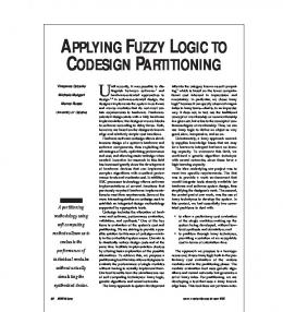
1.2.3 Embedded systems and controllers Embedded systems and controllers are most often characterized by being fixed computer-systems carrying out a specific task which is typically to control some kind of machine. Exceptions are, for example, information-systems such as a wrist watch. Though desirable in some cases, flexibility and ease of reprogramming is most often not of highest priority when designing such systems. Of higher importance is low unit price when mass-produced, reduction of physical size, improvement of reliability and diminishing of power-consumption. The term “embedded system” stems from the fact that such systems are embedded as fixed parts of another larger system in which they typically perform some controlling function. Figure 1.1 shows an example of a typical embedded system. A general embedded system may have dedicated hardware as well as dedicated software running on one, or more, processors in addition to sensors and actuators to interact with the environment. An important class of embedded systems are real-time systems which have to be capable of reacting to exterior events within a fixed time-frame. The missile defense subsystem of a fighter airplane, for instance, has to be capable of producing a defensive response to an incoming missile within the time-interval from missile detection to missile impact, even if it means closing down other lower priority subsystems of the aircraft temporarily. Specific sub-functions of embedded systems can thus have associated with them certain timing constraints which must be satisfied. If the micro-controller cannot perform the sub-function within the specified time-interval, dedicated hardware must be allocated for this purpose.
Sensors
Actuators
Memory
ASIC
Processor Embedded system Environment
Figure 1.1: Essential part of an mixed embedded system [23, page 12, fig. 2]. The optimal constraint conforming distribution of functionality (sub-functions) between the micro-controller and dedicated hardware is a codesign problem as it requires careful analysis of the tasks to be carried out by the embedded system and of the capabilities of the subunits of the system (micro-controller and ASIC in figure 1.1). The aim of codesign in this case will be to obtain the cheapest system which conforms to the specified constraints. The analysis can for example reveal that the micro-controller in a given system could be replaced by a cheaper one with more limited functionality if some parts of the system’s functionality were moved to an ASIC that was required anyway. Or the other way around: one could perhaps settle with a cheaper ASIC if some of its less time-critical functions were moved to the micro-controller.
1.2.4 Software-execution acceleration Most computer-programs would benefit from a speedup. Obvious areas are scientific applications such as whether forecast, image analysis, simulation in nuclear physics and astronomy, etc. But also everyday applications such as word-processing and spreadsheet calculations are good candidates. The classical way to achieve such speedup is to use a more powerful computer, possibly with a dedicated architecture especially suited to the problem. Other common measures are to use more or less general purpose coprocessors such as numeric coproc essors and graphics accelerators. This of course requires that the software applications are aware of the coprocessors and that they have been fine-tuned to utilize the coprocessors in an optimal way. These coprocessors, however, are dedicated to a very limited number of fixed tasks (floating point calculations and graphics oriented calculations in the above example). The emergence of flexible, programmable hardware circuits such as FPGAs (Field Programmable Gate Arrays) which blur the distinction between hardware and software have made it possible to create more general purpose coprocessors that can be used to speedup almost any application. This is possible because the FPGA has the ability to execute operations in parallel and can thus be used to exploit parallelism in parts of the software program. This is in contrast to the microprocessor which is sequential by nature and therefore execute instructions one by one. On the other hand, the FPGA can only implement a very limited amount of functionality as many parallel execution units consume a lot of chip area. This is again in contrast to the microprocessor which has almost unlimited functionality (limited only by the computer system’s available memory). So the codesign problem here consists of obtaining the optimal distribution of functionality between the slow, large capacity microprocessor and the fast, limited capacity FPGA. The aim will either be to obtain the fastest execution with a given FPGA or to satisfy a specific latency constraint with the smallest possible FPGA. This evidently has to be done for every software application, yielding a different FPGA configuration for each application. Of course full custom VLSI chips can also be used for the purpose of speeding up applications. They will typically have more capacity
but on the other hand be more expensive and have larger development times. The emergence of dynamically reprogrammable FPGAs has interesting prospects. They could be reconfigured by all the programs executing in a given system to suit their special needs. This only requires a one-time only analysis of the program in relation to this general coprocessor. Ultimately, a computer operating system may be able to perform a real time analysis of which threads of a computer program are computing intensive or used often, and may chose to execute these on the coprocessor (after appropriate reconfiguration). A system called PAM (Programmable Active Memory) which contains an array of reprogrammable FPGAs has already been built and successfully employed in areas such as cryptography, data compression and simulation of physical systems [23] [2]. It should be noted that this way of speeding up software is closely related to speeding up software by analyzing it for parallelism and distributing program threads amongst processors in a parallel architecture. An important distinction, however, is that such processors are (probably simple) sequential instruction-set processors which do not have the limited capacity problem of the FPGAs.
1.2.5 Hardware emulation and prototyping Just as the usage of dedicated hardware such as FPGAs can speed up general software programs, it can also be used to speed up the simulation of complex digital systems, as this is a task that can be performed by a computer program. A specific advantage of using a FPGA is that it makes it easier to more accurately simulate the execution of hardware parts operating in parallel as the blocks of the FPGA themselves execute in parallel. As this area is just a special case of the software acceleration area, it will not be discussed further here.
1.2.6 Common characteristics The preceding description of different codesign areas reveals some common characteristics. These are summarized below:
� �
�
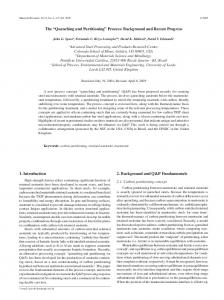
There is a general need of analysis of the total system by estimation and simulation in order to be able to implement each part of the system in a way that makes the total system behave optimally. This in turn means that: The optimal configuration of the system becomes closely dependent on the tasks to be carried out by the system. For each task to be carried out there is an optimal systemconfiguration. For each set of tasks to be carried out either a compromise configuration must be found or the system must be able to adapt (be reconfigured) to each task in turn. As we saw, embedded systems typically have one single task to be optimized for whereas DSP systems typically comprise a set of tasks. Instruction-set processors have to be optimized for a very large range of tasks. These can of course be divided into groups (general purpose computing, scientific computing, control) and within each group typical characteristics of tasks (programs) in the groups must be found by for instance simulation and profiling. There is also a need of means for fast design space exploration. By this is meant the initial choice of system-components before their exact configuration and interconnection has been determined and before the system’s functionality has been distributed amongst them. Figure 1.2 illustrates the importance of means for design space exploration. As seen, there
are many possible combinations of system-components to choose from when constructing a new DSP. An automated tool to aid in the selection would help ensure that the optimal combination is found. (What the phrase optimal really comprises is analyzed in detail later).
� �
The need of the ability to reuse previous designs was most evident in the DSP section, but all areas of codesign will benefit from design for reuse [19]. The need of general retargetable system level simulators.
... 56 K 96 K ...
Analog ... Switched capacitor
Motorola Commercial chip TI
’C25 ’C30 ’C50
Design Commercial core Mixed A/D
ASIC w. DSP core In-house core
Digital
H/W
FSM Random Logic
F/W
Microcode Machine code
Control
Bit-serial Custom architecture
Bit-parallel
Manual Synthesized
Direct map
Figure 1.2: DSP Design Space Alternatives [26, page 16, fig. 3.1].
1.3 General problems and aims of codesign This section tries to characterize the general current codesign development style. The purpose of this is to be able to set up demands to an ideal integrated automated codesign environment.
1.3.1 The traditional approach to codesign Figure 1.3 shows the general design cycle as employed on a manual ad hoc basis. The system description is typically an informal verbal description of required system functionality. Included in the description are functional requirements and constraints. The system must fulfill the functional requirements while conforming to the constraints. The deficiency of this manual method is that the distribution of functionality amongst the components is decided at an early stage. Hereafter the development of each component is initiated, and only after all components have been fully modeled or implemented, can the total system’s functionality be verified. If it does not conform to the system description, the components must be altered or new components must be selected. But meanwhile considerable manpower has been invested in the process. Another problem is that it is very difficult to know whether the optimal system has been chosen.
Select Components
C1
C2
... Cn
System description
Functional description Determine functionality and configuration for each
C1
C2
Constraints
... Cn
Model each component
M1
M2
Model system
... Mn
System model
Simulate and test
No
Implement system
Implement components
I1
Simulate and test
I2
...
In
System
Test
Test
Yes OK?
No
Yes OK?
No
Yes OK?
No
Yes OK?
Final System
Figure 1.3: The ad-hoc development cycle.
1.3.2 The structured approach to codesign The structured codesign approach tries to postpone the decision about choice of system-components and distribution of functionality amongst them to as late a stage as possible. This can be done by describing the system’s functionality in a system-independent language which has the ability to model complex systems consisting of communicating units executing in parallel. Examples of such languages are VHDL, CSP (Communicating Sequential Processes) and ST (Synchronized Transitions). Using formal methods and simulation, this description can then be verified at an early stage and some parts of the system’s functionality can be verified. Design errors and discrepancies between the verbal system description and the formal description can thus be caught at an early stage. When the formal description is verified, it can then be refined towards the final implementation by using transformations which are guaranteed to preserve the functionality of the system. If design specifications change before an actual implementation has been chosen, it is easy to alter the formal description and verify it again.
However, there is still the problem of choosing system components and architecture and of ensuring that system constraints are met. System components and architecture must be chosen in a way so that the system cost is minimized and system constraints are met. Figure 1.4 depicts the structured approach as described above. An advantage of the structured development style is that it can be used to obtain systems which are proven to be correct in accordance with the functional specification. This is indicated below. Much theoretical work however remains to be done in this area. Specification ! Formal specification ! Formal verification ! System independent language formulation ! Cosynthesis ! Correct system.
1.3.3 Constraints, costs and optimality factors As seen in the preceding chapters, constraints and costs are important parts of the system description. Optimality factors are factors that should be optimized for in the design process. Both optimality factors and constraints are expressed in terms of costs. Costs may be either global or local. Examples are listed below. Global costs could be total execution-speed, system price, development time, time to market, physical system dimensions, total power consumption, total thermal and electro-magnetic radiation, environmental impact, etc. Local costs are associated with the individual system components, and include computing speed, throughput rate, component area (physical dimensions), price, power consumption, etc. Constraints can also be either global or local. Examples are: Total price must be less that < maxprice >. Environmental impact should be less than < maximpact >. Second source availability should be better than < availability >. ASIC chip area should be less than < maxarea >. Min. execution-time for < subfunction > should be < mintime >. Optimality factors can also be global as well as local. Examples follow below: Minimize system price. Minimize total execution speed. Maximize execution speed of < subfunction >. Minimize function of system price, development time, environmental impact, power consumption, etc, Minimize area of given component. Minimizing a function of several optimality factors is extremely difficult. The problem is that optimality-factors often compete with each other and with constraints. Maximizing execution speed may imply choosing a fast component, but fast components have a tendency to consume more power than slower components, so such a choice may violate a power-consumption constraint or decrease a power-consumption optimality factor. As seen, designing an optimal system is very difficult as there is a multitude of, often competing, factors to take into consideration. As
a result, manually constructed systems are often not optimal or are too expensive because the designer did not have time to consider a lot of design alternatives. This motivates the construction of automated codesign tools which can help in design-space exploration and system optimization.
(Change verbal or formal description)
Design space (Components)
Verbal description
Optimization goals
Applications
Formal func. description
Constraints
System and component costs
VHDL / ST / CSP
Functional Test
No OK? Yes
Choise of optimal system
Choose a combination of components
Implement total system Determine system cost
Test against constraints.. Repeat if violated
Make models. Simulate and test. Determine system cost estimates
Repeat until a constraint conforming cost optimal solution is found
Implement parts of system. Determine real component costs.
Figure 1.4: The structured development cycle.
Chapter 2 Introduction to HW/SW cosynthesis 2.1 Introduction Binary cosynthesis, which is commonly referred to as Hardware/Software Cosynthesis is the synthesis of a mixed system with only two elements, traditionally denoted the software component (a microprocessor) and a hardware component (Full Custom, ASIC, FPGA, PAL, etc.). This is depicted in figure 2.1. Processor
Communication Channel
ASIC
Figure 2.1: Target system for HW/SW cosynthesis. General n-ary synthesis is synthesis of a mixed system with several hardware and software components. In the most general case, cosynthesis can be regarded as the synthesis of a system with an arbitrary number of processing elements (PEs) which are capable of communicating with each other through communication channels. Examples include computer networks, multiprocessor architectures, etc. The HW/SW systems described above are just special cases. There are many possible combinations of PEs and many different ways of connecting them. Some examples of different architectures are shown in figure 2.2 P1
P2
P3
P4
P1
a) Ring structure
P2
P3
M
b) Bus system with shared memory M
Figure 2.2: General mixed systems. The PEs execute in parallel (to a degree limited by the communication protocol) and can thus exploit the eventual parallelism of the functionality, the system is supposed to implement. Given a functional description, the problem of dividing it into subtasks and determining the distribution of subtasks amongst the different PEs is very complex. For multiprocessor architectures and networks there exist algorithms for workload distribution which try to solve this problem. This is done for systems where the PEs and their interconnect structure are fixed. Another aspect is that the PEs in such systems have virtually unlimited functional capacity (limited by program memory). This simplifies the workload distribution algorithm. But when we add the extra dimensions to the problem to 11
1. determine the optimal number of PEs, 2. determine the optimal interconnect architecture, 3. determine the optimal configuration of the PEs (microprocessor type, microprocessor instruction-set, number of adders, multipliers, etc. on a FPGA/ASIC/Full Custom chip, etc.) and 4. determine the optimal distribution of subtasks amongst PEs where some of them may have very limited capacity. the problem becomes extremely complex. The fact that the PEs operate in parallel adds to the problem complexity. This complexity is the reason for restricting us to only consider the binary cosynthesis problem. Of course, the hardware system and the software system may also execute in parallel in the binary case, but the effects of this are easier to analyze than in the general case. It is, however, important to remember that the binary cosynthesis problem has many parallels to the general problem described above, as it might be possible to utilize previous solutions to problems in related areas of research (network algorithms, etc.).
2.2 The hardware/software distinction This section tries to clarify the distinction between the terms “hardware system” and “software system” as the distinction is no longer as clear as it has been. This is due to the emergence of “programmable hardware circuits” such as FPGAs which blur the distinction between hardware and software. The traditional conception of hardware is that it is fast due to the the inherent parallelism but non-flexible as its functionality is hardwired. Software systems (microprocessors), on the other hand, are slower due to the sequential execution of instructions and very flexible as the system’s functionality can be altered by simply replacing the program. The programmable hardware circuits fall somewhere in the middle of the hardware-software spectrum. This is illustrated in figure 2.3 which also shows other distinctions between the different types of systems. Trade-off
Standard coprocessor
Core coprocessor
ASIP
ASIC
Performance Power Flexibility Design time
Medium High Medium Low (software)
Medium Medium High Medium (hardware, software)
High Medium-low High Higest (hardware, software)
Highest Lowest Low High (hardware)
Figure 2.3: Trade-offs in different design approaches [23, page 11, table 1]. The distinction between hardware and software that will be used in the following in relation to cosynthesis is that software systems (microprocessors) have a fixed architecture and (almost) unlimited capacity while hardware systems (FPGAs, PALs, ASICs, etc) have a flexible architecture which must be determined (synthesized) by the cosynthesis system and have limited functional capacity (on-chip area). ASIPs fall somewhat outside of this classification as they are programmable but also has an flexible architecture (the instruction-set).
2.3 Hardware synthesis High level hardware synthesis is the process of automatic transformation of a pure functional description of an algorithm into hardware which has the same functionality. The functional description can be a specification of a boolean function or a state machine, an algorithm written
in a hardware oriented programming language such as VHDL, CSP and ST, a data-flow graph, etc. The synthesized hardware could be a PLA (Programmable Logic Array), an FPGA (Field Programmable Gate Array), an ASIC (Application Specific Integrated Circuit), an ASIP (Application Specific Instruction-set Processor), a full custom VLSI-chip, etc. High level synthesis encompasses such disciplines as functional partitioning and binding, logic synthesis, floorplanning, placement, routing, layout generation, compaction, etc. Most automatic synthesis systems are targeted at a single hardware platform or at a class of hardware systems with similar characteristics (a range of PALs, different VLSI technologies, etc.) and usually the manufacturer of each synthesis system has provided a wide range of tools (mixed level simulators, routers, etc.) for different steps of the synthesis process. Other systems provide support for several hardware systems. The Synopsys synthesis system [6] can for example produce net-lists for ASICs as well as for FPGAs.
2.4 Software synthesis By software system is meant a system including a traditional programmable microprocessor executing a set of instructions (the software or program). Many tools also exist for the synthesis of software. The synthesis in this connection consists mainly of transforming a high level language description (C, Pascal, Lisp, Fortran, etc.) into a set of microprocessor instructions operating on the different parts of the specific microprocessor (ALU, registers, etc.). This synthesis process is commonly referred to as compilation and is performed by a compiler. Other related tools are debuggers and simulators.
2.5 Motivations for distributing functionality to either hardware or software In many cases the hardware system is supposed to work in conjunction with a software system in which it has the role of performing some computation intensive parts of an algorithm much faster than can be done in software. The role of the software system is in these cases to transfer data to and from the hardware system, specify which functions to perform, analyze the processed data and handle the interface to the exterior world (to users, peripherals, etc.) and finally to execute the non computation intensive parts of the algorithm. The reason for not including the functionality of the hardware system entirely in the software system is that the software system is typically equipped with a general purpose microprocessor with a limited set of operations and therefore may not be sufficiently efficient in performing the required computational task. On the other hand it is cheap because it is produced in large quantities. The hardware system can be faster because it is not bound to a fixed architecture and therefore can be tailored to architecturally match specific parts of the algorithm, to exploit parallelism in the algorithm by letting a number of hardware units work in parallel, have more and/or larger data-paths, etc. This tailoring, however, requires a major effort on behalf of the hardware designer or hardware synthesis tool in order to be implemented optimally. Development of the hardware system must therefore be regarded as expensive compared to development of the software system, even if it is performed by an automatic synthesis tool. Dedicated hardware should therefore only be used if constraints which can not be fulfilled in a software system necessitate it. This complexity of hardware design is one of the reasons for not implementing the software’s functionality entirely in the hardware system — it increases the turnaround time of the design
cycle. Another reason is the limited size of the hardware chip putting a limit to how much functionality there can be on one chip. A third reason is the flexibility and ease of programming of the software system. So when constructing a system with a required functionality, a division into a software part and a hardware part is often inevitable if the system has to meet certain timing-, throughput- and area constraints. Below is listed different motivations for moving parts of a system’s functionality into either hardware or software: Reasons for moving functionality to hardware
�
Faster execution due to architectural flexibility and exploitation of parallelism, etc. May be the only way to achieve required performance with respect to execution speed and throughput rates.
Reasons for not moving functionality into hardware
� � � � � � �
Expensive to develop — Time-consuming to optimize for a specific algorithm. Expensive to produce, especially in small quantities. Difficult to alter once developed. Change of algorithm might dictate a new architecture. This is true for full custom, but but not in the same degree for FPGAs. Difficult and time-consuming to simulate/debug. Communication overhead may be a problem. Changes (new versions) cannot be easily sent to customers as it is possible with software. May consume too much area on the chip(s) available (for both economic and power consumption reasons).
Reasons for moving functionality to software
� � � � �
Relatively cheap to develop. Fast development. Easier to maintain and to alter. Amount of functionality limited only by amount of available RAM, a parameter which is easy to change. Easy to simulate and debug. New software versions can easily be sent to customers.
Reasons for not moving functionality to software
� �
Too slow for some problems due to the general nature of the microprocessor. Communication overhead may be a problem.
2.6 Motivation for binary cosynthesis As stated above, we are in a situation where the design of a large range of systems consists of the simultaneous design of a hardware part and a software part. Such system design will be denoted hardware/software codesign or simply codesign in the following. We are also in a situation where automatic synthesis of individual software systems as well as of individual hardware systems are well researched areas in which a full suite of synthesis tools have been developed. But utilizing these is not enough for optimal hardware/software codesign. When designing on the system level it is, as stated earlier, necessary to view the system as a whole and to consider the interaction between system components. It is necessary to determine the distribution of the system’s required functionality onto hardware versus software and to consider the effects of the communication between hardware and software. In order to be able to perform this task automatically, it is necessary to develop a merge between a silicon compiler and a software compiler which could be denoted a system compiler. This system compiler would take as input a functional description, description of costs, constraints and optimization goals, a description of the software system, the hardware system and the communication media, and produce as output a software program and a synthesized piece of hardware.
2.7 General problems of binary cosynthesis This section tries to evaluate the benefits and drawbacks of binary cosynthesis. In order to be able to do this, an overview of aims and basic problems of codesign is first presented: The aim of codesign (manual as well as automatic) is to achieve a system which is optimal in some sense. Optimality criteria may include timing and throughput rate constraints on specific parts of the system’s functionality or economic criteria such as constraints on hardware/area consumption or software object code size. Of course the global constraints described in section 1.3.3 could also be applied. The problem of codesign when applied to a system with one software component and one hardware component connected by a communication channel is then to achieve an optimal partition of an algorithm (formal description of required system behavior) into software parts and hardware parts. By partitioning is meant the division of the algorithm into smaller pieces and the distributing of these pieces to either hardware or software. The pieces have to be able to communicate with each other, so partitioning implies the addition of communication primitives to both the software pieces and the hardware pieces. Achieving an optimal partition is not a simple task, as the following examples show. Typically, fast pieces (or pieces that are executed few times) are placed in software and slow pieces (or pieces that are executed many times) are placed in hardware, but a specific slow piece may induce a large communication overhead when transferred to hardware which makes the transfer infeasible anyway. Also, a piece that could be beneficially placed in hardware with respect to execution speed could require a relatively large amount of area, thus preventing other pieces from being placed in hardware, even though they might improve system performance much more, were they allowed to be. Another problem is to determine the granularity of partitioning, i.e. the size of the pieces. Yet another problem is that because it is impossible to build an exact computer model of the system on which to distribute the algorithm, the automatic synthesis tool in reality optimizes on a model which may deviate considerably from the real world. Therefore the synthesis tool cannot be expected to reach results which are optimal when applied to the real system. An experienced systems designer may be able to achieve a near optimal partition for some algorithms, while for other perhaps larger algorithms with no apparent partition i t might prove
impossible for a human designer to achieve the optimal partition. Under all circumstances manual system analysis compared to an automatic approach is a time-consuming process which increases the turnaround (or completion) time of system development. On the other hand the experienced system designer may be able to recognize in the algorithm certain larger structures (e.g. FFT calculation, convolution, compression, matrix operations, decoding, etc.) which he knows there have been developed good hardware solutions for, and which he would therefore always place in hardware. In cases like this, it would be difficult for an automatic tool to reach the same performance as the human designer.
2.8 Characterizing the different areas of binary cosynthesis This section tries to characterize the different areas of binary cosynthesis by three types of constraints/optimality factors: Speed, throughput and area. Each of these may be either a constraint or an optimality factor. If it is a constraint, the designer requires it to be fulfilled (e.g. that the algorithm executes in N ms.). If it is an optimality factor, it is a factor that the designer wishes to optimize for (e.g. for area). If we merge the throughput and speed criteria, we have the following combinations of speed and area constraints versus optimality factors: Optimal speed and fixed area constraint: Examples are speedup of existing software solutions with a fixed capacity hardware coprocessor and improving of prototype performance. Optimal area and fixed speed constraint: Embedded systems and DSP systems are obvious candidates for this combination. Combined speed constraint and area constraint: This is the case if a given coprocessor is available and the goal only is to find a partition which satisfies the speed constraint. Examples could again be embedded systems and DSP. Combined optimal speed and area: A partitioning algorithm could for example allow the designer to weigh the speedup factor and the area factor with different percentages. He could then try different combinations of percentages and chose the one which give the best result.
Chapter 3 Problem definition The aims of the project have been to
� � � �
Investigate basic theoretical aspects of hardware/software codesign. Implement a hardware cosynthesis test bench system which can be used to investigate and compare existing and new partitioning algorithms. Characterize and determine benefits and weaknesses of previous work by various research groups. Investigate how partitioning can be improved, and if possible, implement and evaluate such improvements.
17
Chapter 4 Theoretical foundation 4.1 General problems of modelling The basic problem of most areas of optimization is that it is necessary to build a model of the real world problem, optimize within the model domain, and then transform the model domain results back to the real world domain. Results that are optimal within the model domain may not be optimal when transformed to the real world domain and if result A is better than result B in the model domain this may not hold in the real world domain. Clearly it is important to model the real world as closely as possible and it is equally important to always carry out a series of tests in the real world domain when the performance of an algorithm is evaluated. Another problem of algorithm evaluation is that there often exists a fixed set of benchmarks which are used to evaluate the quality of different solutions to a specific problem (both within the model domain and in the real world domain). It must be evaluated how well this set of benchmarks correspond to real world stimuli. These aspects are important to have in mind when reading the report as the work that has been carried out has been done within the model domain. It remains an item for future research to carry out real life evaluations.
4.2 Partitioning models As described in section 4.1, the accuracy of the model used by the partitioning algorithm greatly influences the quality of the result when the partitioned model is transformed back to “the real world” domain. This section presents different models of the hardware/software system, and tries to evaluate the advantages and disadvantages of each. The models are arranged by increasing accuracy with respect to their ability to model the ideal hardware/software system. It should, however, be noted that there is often the choice to implement the system according to the model, so that the model’s presumptions actually become guidelines for how to implement the system. The advantage of this can be that the final physical system behaves more like the model so that estimates of system behavior obtained by estimation and optimization within the model are also good estimates of the physical system behavior. If, for example, hardware/software partitioning has been performed using the very simple model which is described in the first section below, and the system is actually implemented in accordance with a more complex model which takes miscellaneous possible optimizations into consideration (that is, these optimizations are actually performed), it is possible that some constraints are violated in the physical system, even though they were not within the simple model. This problem is especially severe in the case of design 18
of real-time systems where timing constraints must be satisfied. Fortunately, implementing the system in accordance with a more accurate model will in most cases increase performance so that timing constraints are not violated. The opposite situation, that an advanced model is used for partitioning and simplistic model for implementation is even worse — here it is almost guaranteed that timing-constraints are violated. So the designer must assure that the system is implemented in accordance with the employed model, or the implementation of the system must be performed and checked by the system. Before presenting the partitioning models, a note on how the input specification is initially divided into smaller parts is appropriate:
4.2.1 Clustering Clustering is the process of grouping pieces of functionality from the functional specification together in blocks which can be placed in either hardware or software. These pieces are called BSBs which stands for Basic Scheduling Blocks. Several clustering strategies can be imagined: 1. Most fine grained clustering 2. Clustering to < Level > 3. Even sized clustering with max size = < Size > 4. Even sized clustering with max-elements = < Num > 5. One of the above, but never expand < labellist > 6. One of the above, but always expand < labelist > Once a clustering has been determined, partitioning algorithms can be employed in order to determine the best combinations of BSBs to implement in hardware. The following sections present a set of partition models within which the partitioning algorithms can operate.
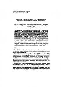
4.2.2 The simple partitioning model Figure 4.1 shows the simple partitioning model. The characteristics of this model are:
� � � �
Fixed clustering of basic scheduling blocks (BSBs). Each BSB has fixed area (ai in the figure) when implemented in hardware, independent of which other BSBs are implemented in hardware. Each BSB receives a constant speedup when implemented in hardware, independent of which other BSBs are implemented in hardware. If a BSB is placed in hardware, its read-set variables are always transferred from the software system to the hardware system prior to execution of the BSB, and its write-set variables are always transferred back to the software system when it has finished its execution.
S/W
H/W
S/W
a1
H/W
a1 t comm1,b2
a2 t comm2,b2
t comm1,b2
t2
a2
t2
t comm2,b2 t comm1,b3
a3 a3
t3
t comm2,b3 a4 a4
a)
b)
Figure 4.1: Simple partitioning model. The last case implies that there will always be a constant execution time
texecution;bi = tcom1;bi + ti + tcom2;bi for a block which is transferred to hardware. This means that we can associate two numbers with each BSB, namely its area and its speedup when implemented in hardware. If the optimization goals are one of the following, the partitioning problem now becomes relatively easy to solve. 1. Optimize for speed with a fixed area constraint. 2. Optimize for area with a fixed speed constraint. Basic Scheduling Blocks t1
t2
t3
a1
a2
a3
...
Basic scheduling blocks tn
a1
a2
a3
an
t1
t2
t3
an ...
Box area equals area constraint
Box area equals exec. time constraint
a)
b)
tn
Figure 4.2: Problem interpretation when optimizing for speed or area. Figure 4.2 shows an interpretation of the partitioning problem for each of the two optimization cases above. The number inside the BSBs corresponds to the area of their boundary box. In a), the problem is to find a combination of BSBs whose area sum is less than or equal to the area limit of the hardware system and whose execution time sum is minimal. In b) the problem is the dual, namely to find a combination of BSBs whose execution time sum is less than or equal to the execution time limit and whose area sum is minimal. So in both cases the problem is to find a combination of BSBs from the dotted box which fits in the solid-lined box and which minimizes the sum of the figures above the small boxes1 . note: Instead of execution times ti , the induced speedup si of moving a BSB to hardware should be used in the figure and in the discussion. 1 Rev.1.1
This problem is a special case of the Knapsack Stuffing problem where a thief is faced with the problem of stuffing his fixed capacity knapsack with valuables from a safe, each of which has a volume and a value, in a way that optimizes his gain. This problem is an NP complete problem which can also be formulated as an ILP (Integer Linear Programming) problem. As is the case with other ILP problems, there exists a solution which is polynomically bound (with respect to the number of observed elements) to one of the variables in the problem [27]. In this case, it can be shown that there exists a solution which has time-complexity O(N � A) and area-complexity O(N ) where N is the number of BSBs and A is the total area (chip-area in case a, “time-area” in case b) [4]. This, however, requires that the areas ai , the execution-times ti and the total area A are integral values. It should be noted that if there exists a bond between N and A, the algorithm complexity could increase. If, for example, the area of BSBn is proportional to 2N , and A must be large enough to contain the largest BSB, the time-complexity becomes O(N � 2N ). In practical applications, the sizes of the individual BSBs will however be independent of the number of BSBs. An advantage of this simple model is that it offers a fast algorithm for solving the two simple problems listed above. This makes it suitable for design space exploration, where the designer can get a fast estimate of how good partitionings he can obtain with a number of different systemconfigurations.
4.2.3 Partitioning model with adjacent block communication As evident in figure 4.1.b, there is an unnecessary communication overhead associated with the communication from BSB2 to BSB3 . In the simple model where we have to be able to associate a fixed hardware execution-time with each BSB, this is inevitable. However, it results in an implementation which is not optimal. It would be better if BSB2 could send its write-set variables directly to BSB3 by storing them in local hardware memory or registers. This model is depicted in figure 4.3.a. S/W
S/W
H/W
H/W
S/W
a1
a1
a1
t comm1,b2
a2
H/W
t2
t comm1,b2
t comm1,b2
a2
a2
t2
a3
t3
a4
t4
t2
t comm2,b2
a3
t3
a3
t comm2,b3
t comm1,b4
a4
a4
a5
a)
t4
t comm2,b4
t comm2,b4
a5
a5
b)
c)
Figure 4.3: Partitioning model with adjacent block communication. The characteristics of this model are
�
Fixed clustering of basic scheduling blocks (BSBs).
� � �
Each BSB has fixed area (ai in the figure) when implemented in hardware, independent of which other BSBs are implemented in hardware. Each BSB receives a constant speedup when implemented in hardware, independent of which other BSBs are implemented in hardware. Adjacent blocks placed in hardware may communicate directly with each other.
So implementing a system according to this model gives better results than implementing it in accordance with the simple model. The problem is that there is no longer associated a fixed execution time with each BSB — the execution-time depends on whether the previous and following block are placed in hardware. Hence, the knapsack stuffing approach is no longer applicable, and more advanced global optimization algorithms of greater time-complexity must be employed. Figure 4.3 b) and c) illustrate how this model can result in a better partitioning than the simple model. Suppose that BSB3 is a relatively small block which receives no speedup when implemented in hardware, while BSB2 and BSB4 receive large speedups. Partitioning within the simple model will then result in the partition in case b), no matter how large the communication overheads tcomm2;b2 and tcomm1;b4 are, as these do not vanish if BSB3 is moved to hardware, as seen in figure 4.1.b. But within the model discussed in this section, it will be beneficial to place BSB3 in hardware, even if it receives no speedup itself, as this will nullify the large communication overhead. This is illustrated in figure 4.3.c.
4.2.4 Partitioning model with general intra-block communication Depending on the data-dependencies given by the CDFG which specifies the functionality to be implemented by the system, it may be the case that not all the write-set variables of BSBi need be transferred to BSBi+1 . If, for example, BSBi writes a variable V which is not used by BSBi+1 but is used by BSBi+3 , and BSBi+1 is placed in hardware, there is no reason to transfer V to hardware prior to executing BSBi+1 . It could be stored in a microprocessor register or RAM from where BSBi+3 could fetch it. Figure 4.4 shows a model in which a given BSB may communicate with all other BSBs and not just with its predecessor and successor BSBs as in the previous model. In this figure, some of the write-set variables of BSB2 are only needed by BSB6 and not by BSB3 . These are denoted V2;6 . If the communication of these variables back to software is very time-consuming, it may be beneficial to allocate a hardware register or hardware RAM to store them temporarily until BSB6 is ready to execute. This reduces the communication time tcomm2;b2 , but not only this. There is no longer the need to propagate the variables V2;6 through BSB3 , BSB4 and BSB5 , so also tcomm1;b5 is reduced. In the same way, storing V3;7 in a microprocessor register or RAM decreases the communication times tcomm1;b5 and tcomm2;b6 This model evidently increases the complexity of the partitioning algorithm which must now also be able to determine the optimal allocation of variables in the hardware system (in the software system unlimited RAM is assumed to be available for this purpose). The area-penalty of allocating some of BSBi ’s write-set variables must be weighted against the resulting speedup of communication of this and subsequent BSBs. The total area of the BSBs which are transferred to hardware no longer equals the sum of the individual BSBs’ area; it depends on register/RAM allocation.
S/W
H/W
1 t comm1,b2
2 t comm2,b2
3 V2,6
Reg/ Mem
4 t comm1,b5
5 Reg/ Mem
V3,7 6
t comm2,b6 7
Figure 4.4: Partitioning model with general intra-block communication.
4.2.5 Partitioning model with global scheduling/allocation The preceding models have presumed that the hardware area of BSBs remains fixed independent of partitioning. This can be obtained in one of the following ways. 1. Global allocation of hardware resources and scheduling of the individual BSBs is performed before partitioning. The fixed hardware area ai of the individual BSBs is then the area of their corresponding hardware controller. 2. Hardware resources are allocated separately for each BSB which is then scheduled as above. This is also done before partitioning. In this way there is no hardware sharing amongst modules which means that a lot of on-chip area is wasted. This waste is proportional to the number of BSBs. The first method is of course to be preferred as it allows for optimal hardware sharing. But especially in connection with reuse it may be beneficial to use the second method. A designer may have built a library (or rather libraries for each possible hardware target sys tem) of often used functions and created implementations of these where the internal structure (controller, datapaths, interconnect) has been optimized. If a BSB corresponds to such a module, it may not be desirable to employ hardware sharing with other BSBs as this would imply disregarding the internal optimal structure of the module. The problem with the approaches presented above is that it is not possible to find an initial allocation which is optimal in terms of hardware sharing for all partitions. In order to optimize hardware sharing, global scheduling must be performed for every partition which is considered during the partitioning process. This means that the sizes and speedups of the individual BSBs which are transferred to hardware are no longer constant, but depends in a complicated way on which other BSBs are transferred to hardware. But even within a specific partition their sizes and execution-times are not constant as these values depend on the choice of allocation and scheduling for this specific partition.
Figure 4.5 shows how three different allocations influence the sizes and executions-times of two very simple BSBs which contain no control-structures and can thus be represented by simple DFGs. Note that the BSBs are not executed in parallel as the figure might suggest — they are just placed beside each other for convenience. AA is shorthand for Allocation Area. It is assumed that the functional units all have area 1. T is the number of time-steps required for execution of each BSB. CA stands for Controller Area, and is a figure proportional to the area of the controller which is required for scheduling each BSB. As the number of states in the controller is proportional to the number of time-steps, CA will be proportional to T. In the figure, CA is just set equal to T for simplicity. DFG for BSB 1 +
DFG for BSB 2
+
* /
*
Allocation 1 *
1 /
Allocation 1 +
2 *
AA = 3
+
* +
T=3 CA = 3
1 +
3 *
AA = 4
+
T=3 CA = 3
1 /
2 +
AA = 6
Scheduling
*
* /
*
1 /
Allocation
Scheduling
Scheduling
+
*
*
+
+
*
*
/
*
/
T=2 CA = 2
T=2 CA = 2
T=2 CA = 2
* T=3 CA = 3
Total CA = 6
Total CA = 5
Total CA = 4
a)
b)
c)
Figure 4.5: Partitioning model with variable sized blocks. The figure reveals the following characteristics of global scheduling/allocation:
� �
�
The sizes and execution times of the individual BSBs which are transferred to hardware depends on the combination and number of functional units which have been allocated. The total controller area (Total CA) becomes smaller as the allocation area AA becomes larger. The latter is relatively independent of the number of BSBs (proportional to the size of the union of the functional unit sets of the BSBs — if these sets have many units in common as is most often the case, the statement is true, otherwise not). The former (Total CA) is proportional to the number of BSBs. This result is however only valid when the controller area is modeled in the simple way described above. Section 6.9.1 will describe a more detailed controller area model. All of the allocated units may not be utilized. This depends on scheduling. Of course it is possible to remove unutilized functional units if scheduling and allocation are performed simultaneously for each partition which is considered during the partitioning process. But if allocation and scheduling are performed before the partitioning process begins, some units may not be required. This is evident in the case where partitioning results in only one BSB being moved to hardware. If space was allocated for many functional units before
the partitioning process started, the partitioning algorithm may have found that there was only room for one BSB (the most time-critical which fitted within the remaining area) in hardware. But if this BSB only required a few functional units, the allocation area (AA) could have been smaller, and this could in turn have allowed for moving one more BSBs to hardware! Evidently there is a need of integration between scheduling/allocation and partitioning. The model presented in this section is consequently a model in which the execution times ti and areas ai of the BSBs are functions of the employed allocation and scheduling AS which is further a function of the performed partition P. This is denoted ti;sa;p and ai;sa;p in figure 4.6. Of course this model can be combined with the the previously presented models so that for instance adjacent BSB communication optimization is also included. S/W
H/W
1 t comm1,b2
a 2,sa,p
t 2,sa,p
t comm2,b2
3 t comm1,b4
a 4,sa,p
t 4,sa,p
t comm2,b4
5
Figure 4.6: Partitioning model with global scheduling/allocation. Figure 4.7 shows two examples of different allocations and the resulting area-sizes for the allocated units and for the BSB controllers. Total available area Controllers
Functional units
a)
Total available area Functional units
Controllers
b)
Figure 4.7: Different area configurations. Configuration a) has a large allocation of functional units which means that the implemented hardware will execute fast due to exploration of parallelism. But this means that the available area for controllers is smaller so that only a limited amount of functionality can be moved to hardware. So the system speedup may not be optimal. Configuration b) has a smaller allocation of functional units, so the functionality that is moved to hardware will execute slower than in case a). On the other hand there is room for more functionality, so the total system speedup may be larger. Clearly it is important to choose an optimal allocation. For a given partition and given total area, there exist an allocation/scheduling which optimizes the global system optimization goal. The converse is also true; for a given allocation/scheduling there exists a partition which optimizes the global system optimization goal. So in order to find the optimal partition one of the following two approaches can be followed
repeat select an allocation/schedule AS and total area A C = cost(optimal_partition(system, AS, A, constraints)) until a minimal cost C is found or repeat select total area A and partition P (P must conform to global constraints) AS = optimal_alloc_schedule(system, P, A) C = cost(partition, AS) until a minimal cost C is found The repeat until loop just indicates the iterative process of a global optimization algorithm — the way it iterates may be much more advanced than indicated above. A genetic algorithm may for instance in the first case select a population of gene strings each containing a random total area and allocation, and then iteratively combine these as to reach an optimal combination. Note that if the partitioning optimization goal is to optimize for e.g. speed with a fixed area constraint, the total area need not be select’ed as indicated above as it is given beforehand. If the goal is to optimize for area with e.g. a fixed speed constraint, the total area need only be selected iteratively in the second algorithm (as the optimal alloc schedule algorithm needs it). In the first algorithm, the determination of total area can be done within the partitioning algorithm. This situation is shown below: repeat select an allocation/schedule AS A = total_area( area_minimizing_partition(system, AS, speed_constraint)) until a minimal area A is found The problem with the second algorithm presented above is that we have not considered how the optimal alloc schedule algorithm chooses an optimal allocation/schedule in relation to a global cost function. A general problem with the approaches presented above is that both the partitioning algorithms and the allocation/scheduling problems are often NP complete algorithms (depending on the employed model), so it is tempting to call the combined problem NP2 complete. One could, however, for example in the last algorithm presented above use the simple knapsack algorithm in the inner optimization loop and a genetic algorithm in the outer loop. This could give a good fast initial indication of the optimal allocation/scheduling. This could then subsequently be used by a more time-consuming partitioning algorithm. A better approach would probably be to apply an algorithm which determines the allocation/scheduling and the partition simultaneously.
4.2.6 Partitioning model with functions Functions are either used to hide a component of a procedural hierarchy or to reuse pieces of code which are used more than one time in the functional description. As this reuse of code can be directly translated to reuse of hardware when BSBs containing function-calls are moved to hardware, a cosynthesis system ought to be able to utilize this possibility of reuse that functions offer. The easiest way to cope with functions is to just expand every function-call. This simplifies the cosynthesis process (the functions simply vanish), but can result in suboptimal partitioning because the partitioning system “thinks” that there is less available area for hardware BSBs than there will be in reality if the functions are not expanded in the implementation. Figure 4.8 illustrates the problems that occur when we try to reuse functions which have been moved to hardware. Functional specification
S/W
Pure
Pure
F
Pure
H/W
F
Pure
Pure
Pure
F
F
Pure
Pure
Figure 4.8: Two HW function instantiations with and without SW comm. The BSBs which are named “pure” contain only simple sequential code — no function calls. The BSBs named F call the function F. The first problem is that the first function instantiation needs to receive variables from software prior to execution and transmit them to hardware afterwards. The second instantiation, however, utilizes that it can receive variables directly from the preceding BSB and transmit them directly to the following BSB. Thus, we can not implement a single version of the function — we need one which communicates with software and one which does not. There are four combinations of communication to/from software, so we could of course always implement four versions of the functions, but this would be wasteful. It would, however, be a simple solution which requires no extra special hardware control. It should be noted that this problem does not occur in the simple model described earlier. Here variables are always transmitted from/to software. The second problem is that there is only a area-penalty associated with the first function-call which is transferred to hardware. Figure 4.9 shows how these problems can be handled within the more advanced HW/SW communication models. For function-call number N, a corresponding hardware block FcommN is created. This block is responsible for receiving variables from either hardware or software and for transmitting variables to either hardware or software. Besides, it must call the hardware implementation of the function Fimpl . The execution-times of these blocks is set to the execution-time of the function. The area of the first block Fcomm1 is set to the sum of its own area and Fimpl ’s area. The area of
Functional specification
S/W
Pure
Pure
H/W
a = a(Fcom1) + a(Fimpl) F com1
F
Pure
F impl
Pure
Pure
Pure
F
F com2 a = a(Fcom2) + 0
Pure
Pure
Pure
Pure
Figure 4.9: Implementing function calls in hardware. subsequent Fcomm modules is set to their own area. This area could be set to zero. This implementation scheme thus means that the area of a function-call BSB can assume one of two values, which can make it difficult for some partition algorithms to handle. Another problem that occurs in connection with functions is that it might be desirable to only implement part of the functions in hardware. If the partitioning algorithm decides that the same part (a computation intensive loop for example) of two function call BSBs should be implemented in hardware, this part should be reused. The reason that the partition algorithm does not always decide to implement the same parts of a given function in hardware is that which parts of a function are computation intensive can depend on the function arguments. An example is the following function. void fun(int a, int b) { for (int i=0; i BestSpeedup[I-1, A] then f BestSpeedup[I, A] = BSBSpeedup + BestSpeedup[I-1,A-BSBArea]; BestChoice[I,A] = I;
g
else f BestSpeedup[I, A] = BestSpeedup[I-1, A]; BestChoice[I, A] = BestChoice[I-1, A];
g
g
g
g
g /* Algorithm */
Algorithm 3: Simple Knapsack Stuffing partitioning algorithm.
Knapsack-reconstruct (NumBSBs; AvailableArea; BestSpeedup[ ]; BestChoice[ ]) �
f
/* Initialization */ fg; HwBSBList /* The best execution-time on the given area has been found. The same execution-time */ /* may be achievable for a smaller area. Reconstruct the BSB combination */ /* that lead to best execution-time while occupying the smallest area. */ 0; AStart false; Found while (AStart BestSpeedup[G, A] then f BestSpeedup[G,A] SeqSpeedup; SLowBSB;HighBSB; BestChoice[G,A]
g
g
else f /* Also assume that the best solution for sequences up to LowBSB-1 */ /* on the remaining area is selected. */ if SeqSpeedup + BestSpeedup[LowBSB-1, A-SeqArea] > BestSpeedup[G, A] then f BestSpeedup[G,A] SeqSpeedup + BestSpeedup[LowBSB-1, A-SeqArea]; SLowBSB;HighBSB; BestChoice[G,A]
g
g
g
g
/* For each area, now see if the best solution found for sequences without */ /* the element HighBSB is better than the solution just found for sequences */ /* with HighBSB. If so, replace the just found solutions with the previously */ /* found better solutions. */ if (HighBSB > 1) 0 to AvailableArea do for all areas A if BestSpeedup[G-1, A] > BestSpeedup[G, A] then f BestSpeedup[G, A] BestSpeedup[G-1, A]; BestChoice[G, A] BestChoice[G-1, A];
g g /* for all groups */
return BestChoice[]; return BestSpeedup[]; g /* Algorithm */
Algorithm 5: PACE - A Partitioning Algorithm with Communication Emphasis.
PACE-reconstruct (NumBSBs; AvailableArea; BestSpeedup[]; BestChoice[]) �
f
/* Initialization */ HwBSBList fg; /* The best execution-time on the given area has been found. The same */ /* execution-time may be achievable for a smaller area. Reconstruct the */ /* sequences that lead to best execution-time, occupying the smallest */ /* area. */ AStart 0; false; Found while (AStart R1 (12) NOP M[?]-->R2 (12) M[?]-->M[1] (24) NOP M[?]-->M[2] (24) M[?]-->M[3] (24) Add M[2],M[1]-->M[1] (32) M[1],R2-->R2 (170) Mult M[2],R2-->R2 (82)
Remembering that NOP nodes are implemented as MOV instructions, it is clear that the first five NOP mnemonics correspond to the first five initializations of the VHDL code (their execution times are calculated as the MOV execution time, even though they are showed as NOPs). The following Add, Div and Mult operations clearly perform the two last calculations of the VHDL code. Notice that register allocation works correctly. The ExtraRegs line of the technology file was set to two, so only two registers are available. Note that the g variable in R[2] is no longer needed after the Div operation, so it is reused for the result. The Mult instruction can be used to demonstrate that the correct addressing mode specific instruction execution times are calculated. Checking the 68000 technology file reveals that the MUL DIRECT MEM, REGISTER to REGISTER instruction takes 82 clock cycles. This is also the number shown in parentheses after the Mult instruction above. If the instruction execution times above are added together, a total of 380 clock cycles is the result. This is the number shown as SWT in the “Estimates” line of the BSB. Verification of hardware execution time estimation The hardware execution time for the first DFG is shown as HWT=11. This means that the DFG has been scheduled to be executed in 11 time steps. Graphical viewing of scheduled dataflow graphs has confirmed that the correct number is calculated from the ALBATRESA annotations. Verification of hardware controller area estimation Using the notation of formula 6.4, page 63, and data from the LIBFPGA hardware library, we have for the first DFG in the example that k = 11 (HWT from above), n = 16, Aflipflop = Aand-gate = Aor-gate = Ainv-gate = 1. Inserting these values in the formula yields
Adecoder = 1 + 1 + 1 + log2 (16) � 1 + (16 ? 1) � (2 � 1 + 1) = 52 This is the same area that has been estimated for the DFG (HWA = 52). Verification of communication time estimation From the “R-vars” line of the branch body 2 DFG we derive a total of 90+90 = 180 readset variable transfers. From the “W-vars” line we have a total of 90 writeset variable transfers. Using the notation of formula 6.7, page 69, we have that NR = 180, NW = 90, TMOV DIRECT MEM,DIRECT MEM = 24, TIMPORT = 1, TEXPORT = 1. This yields the total communication time of the DFG: Tcomm = (180 + 90) � 24 + 180 � 1 + 90 � 1 = 6750 Adding the RCT and WCT entries of the branch body 2 DFG yields 4500+2250 = 6750 as calculated above. Verification of hierarchical BSB calculations From the listing it is easy to be convinced that estimates are added correctly together for child BSBs as to reach the totals for their parents.
7.2 Experiments All experiments were performed on a manually profiled TaoDFG which was translated from the VHDL program big.vhdl shown in appendix G. The dataflow graph was partitioned using different allocations and microprocessor technologyfiles as described in the following sections. The resulting hierarchy contained 36 leaf BSBs which meant that partitioning only took about two minutes with the PACE algorithm.
7.2.1 Tests and comparison of the partitioning algorithms A series of tests have been carried out in order to investigate the performance of the simple Knapsack Stuffing algorithm and of the PACE algorithm. The allocation- and optionfiles files that were used for this experiment are listed in appendix H.1.2. A general note to all the graphs that are presented is that IC stands for the IGNORE COMM estimationmodel, SB for the SINGLE BLOCK COMM estimation model and AB for the ADJACENT BLOCK COMM estimationmodel. The Knapsack Stuffing can perform partitioning according to either the IC or the SB estimationmodel. When partitioning according to the IC model, the communicationtime of a BSB is set to zero, so the BSB‘s total hardware executiontime is assumed to be its raw hardware executiontime. When partitioning according to the SB model, the hardware executiontime of a BSB is the sum of its raw hardware executiontime and its software-hardware and hardware-software communicationtimes. In both cases the BSB has a constant executiontime. The PACE algorithm only partitions according to the AB estimationmodel. This means that it assumes that adjacent blocks have smaller communicationtimes than the sum of the individual blocks’ communicationtimes. The Knapsack algorithm partitioning according to the IC model can have its resulting partition evaluated according to either the IC, the SB or the AB estimationmodels. This corresponds to choosing another implementation than the partitioning algorithm has modeled. Likewise, the Knapsack algorithm partitioning according to the SB model can have its resulting partition evaluated according to the SB or the AB estimation models. For the PACE algorithm it only makes sense to evaluate according to the AB algorithm. Knapsack algorithm - IGNORE_COMM model 5500000 IC-IC IC-SB IC-AB
5000000 4500000
Resulting clockcycles
4000000 3500000 3000000 2500000 2000000 1500000 1000000 500000 1200
1300
1400
1500
1600 Total chip area
1700
1800
1900
2000
Figure 7.1: The Knapsack algorithm ( IGNORE - COMM ) evaluated with three estimation models.
The first graph in figure 7.1 shows the results of the simple knapsack algorithm partitioning according to the IC model. Partitioning has been carried out for all total hardware ares from 1200 to 2000 in steps of 20. The IC-IC graph shows the results evaluated according to the IC model. This graph shows how good a result, the algorithm “thinks” it has achieved. The IC implementation is not realistic as the hardware blocks have to communicate with software. The IC-SB graph shows the result evaluated according to the SB model. As shown, the result of partitioning are far from as good as the algorithm “thinks” if the partition is implemented with the SB model. The IC-AB shows the result evaluated according to the AB estimationmodel, i.e. where intra-block communication is modeled. This better implementation of course gives better results, but far from as good as the algorithm “thinks”. Knapsack algorithm - SINGLE_BLOCK_COMM model 3200000 SB-SB SB-AB
3100000 3000000
Resulting clockcycles
2900000 2800000 2700000 2600000 2500000 2400000 2300000 2200000 1200
1300
1400
1500
1600 Total chip area
1700
1800
1900
2000
Figure 7.2: The Knapsack algorithm ( SINGLE - BLOCK - COMM ) evaluated with two estimation models. The graph in figure 7.2 shows the results of the Knapsack stuffing algorithm partitioning according to the SB model. The results are evaluated according to both the SB and AB estimationmodels. As shown, the results are coinciding. This is because the knapsack algorithm in this case is very reluctant to placing blocks in hardware, as many of the blocks have communicationoverheads which are larger than the speedup they induce. Therefore only a few blocks are placed in hardware. The graphs show the same results because no adjacent block were placed in hardware. When there are no adjacent blocks, the SB and AB estimationmodels give the same result. The graph in figure 7.3 shows the results that can be obtained with the PACE algorithm. As seen, it reaches better results than the knapsack stuffing algorithm for all areas. This is more evident in the following graph. The graph in figure 7.4 shows the results of the two Knapsack Stuffing algorithm implementations and the PACE algorithm, all estimated according to the best estimationmodel AB. So this graph compares the results of the algorithms when their produced partitions are implemented in the best possible way (that we are able to model). As expected, the PACE algorithm yields the best results for all areas as its results are optimal within the AB estimationmodel. But interestingly, the Knapsack algorithm which ignores communication totally (shown as the IC-AB graph) for some areas yields results that are comparable to the results of the PACE algorithm (but for other areas the PACE algorithm yields much bet-
PACE algorithm - ADJACENT_BLOCK_COMM model 3500000 AB-AB
3000000
Resulting clockcycles
2500000
2000000
1500000
1000000
500000 1200
1300
1400
1500
1600 Total chip area
Figure 7.3: The PACE algorithm evaluated with the model.
1700
1800
1900
2000
ADJACENT- BLOCK - COMM
estimation-
Comparison of the algorithms - ADJACENT_BLOCK_COMM model 5500000 IC-AB SB-AB AB-AB
5000000 4500000
Resulting clockcycles
4000000 3500000 3000000 2500000 2000000 1500000 1000000 500000 1200
1300
1400
1500
1600 Total chip area
1700
1800
1900
2000
Figure 7.4: Comparison of the performance of the algorithms according to the BLOCK - COMM estimationmodel.
ADJACENT-
ter results). The Knapsack algorithm which includes communication (the SB-AB graph), also comes close to the performance of the PACE algorithm for some areas, but for other areas its results are much worse. The conclusion from this test must be that partitioning within a model which ignores communication totaly or only models it locally on BSB level mostly yields results that are worse than the results that can be obtained with an algorithm which models communication more globally on an adjacent block basis. Sometimes good results can be reached with the simple models, but there is no general rule for this. If communication is modeled, it should be modeled properly by recognizing the communication speedups that are induced by hardware blocks being able to communicate directly with each other. It cannot be concluded whether the Knapsack algorithm which ignores communication is better than the one which includes communication (although for other tests, the one which ignored communication gave the best results for all areas compared to the one which partitioned according to the SB model). The tests also demonstrate that the PACE algorithm performs much better than the two versions of the Knapsack stuffing algorithm due to the fact that it recognizes adjacent block communication speedup, even though it does not partition all branches and loops optimally. The conclusions presented in this section are therefore still valid. It should be emphasized that these results are obtained within the model domain. Future work should try to transform the results to the real world domain and see whether the results still hold. However, the results do demonstrate that it is important to include the communication aspect in partitioning.
7.2.2 Tests with different allocations In order to test how different allocations can influence the result of partitioning, partitioning has been carried out for three different allocations. The graph in figure 7.5 shows the resulting system performance for each of these. The PACE algorithm was used for partitioning. See appendix H.1.3 for details. The PACE algorithm employed on three different allocations. 3500000 Allocation A Allocation B Allocation C 3000000
Resulting clockcycles
2500000
2000000
1500000
1000000
500000
0 400
600
800
1000
1200 Total chip area
1400
1600
1800
2000
Figure 7.5: Resulting system executiontime for different allocations. The most important modules of allocation A are (add-sub-comb:2, div-comb:1, mulcomb:1). For allocation B they are (add-sub-comb:1, div-ser:1, mul-ser:8) and for allocation
C (add-sub-comb:1, div-ser:1, mul-ser:1). The numbers after the colons indicate how many instances of each module were allocated. The ASAP allocation for the dataflowgraph was (add:9, mul:8, div:2). This information was dumped by the ALBATRESA scheduler. Note that the partitioning results are horizontal (corresponding to an all-software solution) until the specific allocationarea is reached. The graph clearly demonstrates that it is important to choose an optimal allocation, and that which allocation is optimal depends on the available area. It can also been concluded that the performance of a real-world implementation of a given partition depends on which allocation the synthesis tool chooses to employ. If the partitioning algorithm incorporates means of finding the optimal allocation, an external synthesis tool must use the same allocation. This comes automatically if the synthesis tool is part of the cosynthesis system. If an external synthesis tool is used and the partitioning algorithm does not itself find an optimal allocation, the external synthesis tool should attempt to find an allocation that optimizes for the same optimization goals as the partitioning system.
7.2.3 Tests with different processors In order to demonstrate how the PALACE system can be used for quick design space exploration, partitioning has also been employed for four different processors. The PACE algorithm was used for partitioning. See appendix H.1.4 for details. The PACE algorithm employed on four different processors. 5000000 8086 68000 68020 80286
4500000 4000000
Resulting clockcycles
3500000 3000000 2500000 2000000 1500000 1000000 500000 0 1000
1100
1200
1300 Total chip area
1400
1500
1600
Figure 7.6: Resulting system executiontime for different processors. The graph in figure 7.6 shows the resulting system performance for each of the modeled microprocessors. If, for example, at an total available area of 1200 it is important to ensure that the executiontime of the algorithm is less than 1000000 clockcycles, the 68020 or the 80286 microprocessor must be chosen (assuming that the optimal allocation has been chosen). An extra price criteria could determine which processor should be chosen. If these microprocessors are too expensive, another solution may be to invest in a larger hardware chip (or a faster one). If the total area is for instance 1300, both the cheaper 68000 and 8086 microprocessors can yield the desired result. Figure 7.7 shows the speedup in percent that could be reached with the four microprocessors. It shows that the slowest processors receive the largest percentwise speedup. A theory has
The PACE algorithm employed on four different processors. 6000 8086 68000 68020 80286
5000
Speedup in percent
4000
3000
2000
1000
0 1000
1100
1200
1300 Total chip area
1400
1500
1600
Figure 7.7: Speedup in % for different processors. been that the larger processors receive the largest percentwise speedup because they communicate more efficiently (using faster MOV operations) but the graph does not confirm that theory. Perhaps the theory holds for the simple SB communication model where communication time is more dominant, but results have not been produced for this model.
Chapter 8 Directions for future work The codesign research area is like a Pandora’s Box. For each new problem which is attempted solved, many new problems seem to emerge. Codesign is a kind of super-discipline which combines several well known research ares. Many problems in these areas are NP-complete. As these problems are combined in codesign (the NP-complete scheduling/allocation problem is combined with the NP-complete problem of finding an optimal machine code implementation of a software program and with the NP-complete problem of partitioning itself), the resulting codesign problem becomes extremely complex. Also, new problems within the well known research areas need to be solved. For instance it suddenly becomes necessary to be able to estimate the area contribution of the hardware implementation of a program fragment before synthesis is even attempted. The challenges of the codesign problem are thus considerable. It is therefore not difficult to think of numerous improvements to the PALACE system and of future research topics. The following is a list of some of these.
� � � � � �
�
More optimal partitioning models should be implemented. Global optimization algorithms which can handle such models should be implemented. Their performance should be evaluated with the PACE algorithm. It should also be possible to optimize for area under a fixed time constraint or under several local time constraints. Perhaps a power consumption constraint should also be supported. This would be relevant for portable systems. Algorithms to find the best allocation should be included (and preferably integrated with the partitioning algorithms). The influence of granularity of clustering on the partitioning result should be examined for the different algorithms. A preselection scheme that always places those blocks in software which are guaranteed (within all partitioning models) to induce no speedup when moved to hardware should be implemented. This would limit the number of blocks which are considered for hardware and thus speed up partitioning. Partitioning’s dependence on the clock frequency should be examined as scheduling can deliver different results depending on how large the cycle time is compared to the propagation delays of hardware modules. 99
� � � � � �
The sensitivity of the partitioning algorithms to the models’ deviations from the real world should be examined. This could be done by gradually making the models worse and examining how this influences the partitioning result. Better software, hardware and communication models should be implemented and investigated. The controller area model should be evaluated on a real world example. It should be examined how current synthesis systems implement controllers. Interconnect area models should be developed. A system that carries out automatic design space exploration given both local and global constraints should be developed. A real world system corresponding to the modeled system should be implemented and model domain results should be compared to real world domain results.
Chapter 9 Conclusion A study of the current state of the new codesign research area has been carried out. Previous work of different research groups which have examined the codesign problem has been based on widely different system models and optimization goals which has maked it difficult to compare and evaluate their results. Therefore a unified set of partitioning models and goals has been derived. A graphical representation of these models which makes it easy to compare the models’ characteristics has been presented. In order to be able to examine current and future partitioning algorithms, a test bench system called PALACE1 has been constructed. For this system, a hardware library for an Actel ACT 3 FPGA and microprocessor characterization libraries for four different processors have been developed. Also, a simple Knapsack Stuffing partitioning algorithm and a novel partitioning algorithm called PACE2 which recognizes that adjacent hardware blocks can communicate directly with each other have been implemented. By comparing the results of the PACE algorithm with the results of the simple Knapsack Stuffing algorithm within the PALACE environment, the danger of using simplified partitioning models and the importance of including the communication aspect in partitioning has been demonstrated. These results are valid despite the fact that the PACE algorithm has proven unable to optimize hardware inter-block communication optimally in certain situations. For the first time (to the author’s knowledge) a hardware area model which calculates with a fixed allocation area and, for each hardware block, a variable controller area, has been utilized in partitioning. This has made it possible to examine how choice of allocation influences partitioning. Partitioning with three different allocations has shown that the partitioning result is closely dependent on the chosen allocation. Methods for choosing an optimal allocation should therefore be employed. Finally, by examining partitioning results for the four different processor models, it has been demonstrated how a partitioning system can be used for quick design space exploration at an early stage in system development. Lyngby, October 16, 1995 Peter Voigt Knudsen
1 Partitioning ALgorithm Analysis 2 Partitioning Algorithm with
and Comparison Environment. Communication Emphasis.
101
Acknowledgements I would like to thank my supervisors Jan Madsen and Robin Sharp for inspired and inspiring guidance and for the many fruitful discussions we have had. Also, Jesper Grode deserves a warm thank for always being willing to enlighten me on details of his work and for being helpful with many practical details. Jan Madsen is assistant professor, Robing Sharp is associate professor and Jesper Grode is M.Sc. All three are employed at the Department of Computer Science at the Technical University of Denmark.
102
Bibliography [1] Actel Corporation. FPGA Data Book and Design Guide, 1994. [2] P. Bertin, D. Roncin, and J.Vuillemin. Introduction to programmable active memories. In J. McCanny, J. McWhirter, and E. Schwartzlander, editors, Systolic Array Processors. Prentice Hall, Englewood Cliffs, N.J., 1989. [3] Jens P. Brage. A dfg language for the tao system. Version 1.0, 31. July 1993. [4] Thomas H. Corman, Charles E. Leiserson, and Ronald L. Rivest. Introduction to Algorithms. MIT Press, Cambridge, Massachusetts, 1992. [5] Rolf Ernst, Wei Ye, Thomas Benner, and J¨org Henkel. Fast timing analysis for hardware/software co-design. In ICCD ’93, 1993. [6] ES2, editor. ES2 Synopsys Design Kit User Guide. ES2 European Silicon Structures, 1993. [7] Jie Gong, Daniel D. Gajski, and Sanjiv Narayan. Software estimation from executable specifications. Technical Report ICS-93-5, Dept. of Information and Computer Science, University of California, Irvine, Irvine, CA 92717-3425, March 8 1993. [8] Jesper Grode. ALBATRESA documentation, as a HTML-document. On World Wide Web : http://www.id.dtu.dk/˜ dag/Students/jnrg/ALBATRESA.html, 1995. [9] Jesper Grode. ConGIF documentation, as a HTML-document. On World Wide Web : http://www.id.dtu.dk/˜ dag/Students/jnrg/ConGIF.html, 1995. [10] Jesper Grode. Scheduling of control flow dominated data-flow graphs. Master’s thesis, Technical University of Denmark, 1995. [11] Rajesh K. Gupta and Giovanni De Micheli. System synthesis via hardware-software codesign. Technical Report CSL-TR-92-548, Computer Systems Laboratory, Stanford University, October 1992. [12] Bjarne G. Hald. ACE - An Architectural Construction Environment. DAG Documentation System, Technical University of Denmark, 0.26 edition, October 1994. [13] John P. Hayes. Computer Architecture and Organization. McGraw-Hill, second edition, 1988. [14] J¨org Henkel, Rolf Ernst, and Thomas Benner. Hardware-software partitioning for microcontroller design with simulated annealing. In ICCAD ’93, 1993, category 13: Issues in system design. 103
[15] D. Herrmann, J. Henkel, and R. Ernst. An approach to the adaptation of estimated cost parameters in the cosyma system. In CODES ’94, 1994. ¨ [16] Axel Jantsch, Peeter Ellervee, Johnny Oberg, Ahmed Hermani, and Hannu Tenhunen. A case study on hardware/software partitioning. In Proceedings of the IEEE Workshop on FPGAs for Custom Computing Machines, April 1994. ¨ [17] Axel Jantsch, Peeter Ellervee, Johnny Oberg, Ahmed Hermani, and Hannu Tenhunen. Hardware/software partitioning and minimizing memory interface traffic. In EURO-DAC ’94, 1994. ¨ [18] Axel Jantsch, Peeter Ellervee, Johnny Oberg, Ahmed Hermani, and Hannu Tenhunen. A software oriented approach to hardware/software codesign. In Proceedings of the Poster Session of the International Conference on Compiler Construction, April 1994. [19] Claudionor Nunes Coelho Jr., Chih-Yuan Jerry Yang, Vincent Mooney, and Giovanni De Micheli. Redesigning hardware-software systems. In Third International Workshop on Hardware/Software Codesign, pages 116–123, September 1994. [20] Asawaree Kalavade and Edward A. Lee. A global criticality/local phase driven algorithm for the constrained hardware/software partitioning problem. In Third International Workshop on Hardware/Software Codesign, pages 42–48, September 1994. [21] Ludovic Larzul. Translation from vhdl to data flow graph. Master’s thesis, Technical University of Denmark, July 1994. [22] Jan Madsen. Quenya documentation, as a HTML-document. On World Wide Web : http://www.id.dtu.dk/˜ dag/Alien/Quenya.html, 1994. [23] Giovanni De Micheli. Computer-aided hardware-software codesign. 14(4):10–16, August 1994.
IEEE Micro,
[24] Stefan N¨aher. LEDA User Manual. Max-Planck-Institut f¨ur Informatik, Im Stadtwald D6000 Saabr¨ucken, third edition, 1992. [25] Kunle A. Olukotun, Rachid Helaihel, Jeremy Levitt, and Ricardo Ramirez. A softwarehardware cosynthesis approach to digital system simulation. IEEE Micro, 14(4):48–58, August 1994. [26] Pierre G. Paulin, Clifford Liem, Trevor C. May, and Shailesh Sutarwala. Dsp design tool requirements for embedded systems: A telecommunications industrial perspective. Journal of VLSI Signal Processing: JVSPIV005, 1993. [27] Alexander Schrijver. Theory of Linear and Integer Programming. John Wiley and Sons, New York, 1987. [28] Frank Vahid, Jie Gong, and Daniel D. Gajski. A binary-constraint search algorithm for minimizing hardware during hardware/software partitioning. In EURO-DAC ’94, pages 214–219, 1994.
List of Figures : : : :
4 6 7 10
Target system for HW/SW cosynthesis. : : : : : : : : : : : : General mixed systems. : : : : : : : : : : : : : : : : : : : Trade-offs in different design approaches [23, page 11, table 1].
:::::::::::::::::::::::::::::: :::::::::::::::::::::::::::::: ::::::::::::::::::::::::::::::
11 11 12
4.1 4.2 4.3 4.4 4.5 4.6 4.7 4.8 4.9 4.10
Simple partitioning model. : : : : : : : : : : : : : : : : Problem interpretation when optimizing for speed or area. : Partitioning model with adjacent block communication. : : Partitioning model with general intra-block communication. Partitioning model with variable sized blocks. : : : : : : : Partitioning model with global scheduling/allocation. : : : Different area configurations. : : : : : : : : : : : : : : : Two HW function instantiations with and without SW comm. Implementing function calls in hardware. : : : : : : : : : Model for BSBs which contain function-calls. : : : : : : :
: : : : : : : : : :
: : : : : : : : : :
: : : : : : : : : :
: : : : : : : : : :
: : : : : : : : : :
: : : : : : : : : :
: : : : : : : : : :
: : : : : : : : : :
: : : : : : : : : :
: : : : : : : : : :
: : : : : : : : : :
: : : : : : : : : :
: : : : : : : : : :
: : : : : : : : : :
: : : : : : : : : :
: : : : : : : : : :
: : : : : : : : : :
: : : : : : : : : :
: : : : : : : : : :
: : : : : : : : : :
: : : : : : : : : :
20 20 21 23 24 25 25 27 28 29
6.1 6.2 6.3 6.4 6.5 6.6 6.7 6.8 6.9 6.10 6.11 6.12 6.13 6.14 6.15 6.16 6.17 6.18 6.19 6.20 6.21 6.22 6.23 6.24 6.25 6.26 6.27 6.28
Software system components : : : : : : : : : : : : : : : : : : : : : : : : : : : : External and internal transformations of the input DFG : : : : : : : : : : : : : : : ConGIF representation of a simple algorithm : : : : : : : : : : : : : : : : : : : : Hierarchical BSBs and their links to ConGIF : : : : : : : : : : : : : : : : : : : : BSB hierarchy for the ConGIF graph example. : : : : : : : : : : : : : : : : : : : Expansion to level 1 : : : : : : : : : : : : : : : : : : : : : : : : : : : : : : : : Expansion to level 3 : : : : : : : : : : : : : : : : : : : : : : : : : : : : : : : : Ideal software estimation system. : : : : : : : : : : : : : : : : : : : : : : : : : : Two different estimation models [7, page 5, fig. 2]. : : : : : : : : : : : : : : : : : execution-time of a generic instruction for different processors [7, page 6, fig.3]. : : : Example of different dataflow-graph linearizations. Partly from [11, page 27, fig. 10]. Sample allocation-file. : : : : : : : : : : : : : : : : : : : : : : : : : : : : : : : Register transfers for a simple dataflow-graph. : : : : : : : : : : : : : : : : : : : Hardware controller tasks. : : : : : : : : : : : : : : : : : : : : : : : : : : : : : A control unit based on a sequence counter [13, page 301, fig. 4.13]. : : : : : : : : : A modulo-k sequence counter [13, page 300, fig. 4.11]. : : : : : : : : : : : : : : : A 1/2 decoder. : : : : : : : : : : : : : : : : : : : : : : : : : : : : : : : : : : : A 1/8 decoder derived from 1/2 decoders : : : : : : : : : : : : : : : : : : : : : : Area relationships. : : : : : : : : : : : : : : : : : : : : : : : : : : : : : : : : : Read- and writeset analysis for the branch construct. : : : : : : : : : : : : : : : : Read- and writeset analysis for the loop construct. : : : : : : : : : : : : : : : : : Components of a partSysEstimator instance. : : : : : : : : : : : : : : : : : : : : Estimation of a partition. : : : : : : : : : : : : : : : : : : : : : : : : : : : : : : Estimation of a list of adjacent BSBs. : : : : : : : : : : : : : : : : : : : : : : : : Estimation of a single BSB. : : : : : : : : : : : : : : : : : : : : : : : : : : : : : The simple partitioning model used by the Knapsack Stuffing algorithm. : : : : : : : Example of partitioning problem with communication cost considerations. : : : : : : The PACE algorithm employed for a simple example. : : : : : : : : : : : : : : : :
: : : : : : : : : : : : : : : : : : : : : : : : : : : :
: : : : : : : : : : : : : : : : : : : : : : : : : : : :
: : : : : : : : : : : : : : : : : : : : : : : : : : : :
: : : : : : : : : : : : : : : : : : : : : : : : : : : :
: : : : : : : : : : : : : : : : : : : : : : : : : : : :
: : : : : : : : : : : : : : : : : : : : : : : : : : : :
: : : : : : : : : : : : : : : : : : : : : : : : : : : :
: : : : : : : : : : : : : : : : : : : : : : : : : : : :
: : : : : : : : : : : : : : : : : : : : : : : : : : : :
: : : : : : : : : : : : : : : : : : : : : : : : : : : :
: : : : : : : : : : : : : : : : : : : : : : : : : : : :
: : : : : : : : : : : : : : : : : : : : : : : : : : : :
: : : : : : : : : : : : : : : : : : : : : : : : : : : :
: : : : : : : : : : : : : : : : : : : : : : : : : : : :
: : : : : : : : : : : : : : : : : : : : : : : : : : : :
: : : : : : : : : : : : : : : : : : : : : : : : : : : :
: : : : : : : : : : : : : : : : : : : : : : : : : : : :
: : : : : : : : : : : : : : : : : : : : : : : : : : : :
: : : : : : : : : : : : : : : : : : : : : : : : : : : :
36 37 40 41 42 43 44 45 47 48 51 58 59 60 60 61 62 62 63 67 68 71 71 72 72 77 81 83
7.1 7.2 7.3 7.4 7.5 7.6 7.7
The Knapsack algorithm ( IGNORE - COMM ) evaluated with three estimation models. : : : : : : : : : : : : : The Knapsack algorithm ( SINGLE - BLOCK - COMM ) evaluated with two estimation models. : : : : : : : : : : The PACE algorithm evaluated with the ADJACENT- BLOCK - COMM estimationmodel. : : : : : : : : : : : : : Comparison of the performance of the algorithms according to the ADJACENT- BLOCK - COMM estimationmodel. Resulting system executiontime for different allocations. : : : : : : : : : : : : : : : : : : : : : : : : : : : Resulting system executiontime for different processors. : : : : : : : : : : : : : : : : : : : : : : : : : : : Speedup in % for different processors. : : : : : : : : : : : : : : : : : : : : : : : : : : : : : : : : : : :
: : : : : : :
: : : : : : :
: : : : : : :
: : : : : : :
: : : : : : :
: : : : : : :
: : : : : : :
93 94 95 95 96 97 98
1.1 1.2 1.3 1.4
Essential part of an mixed embedded system [23, page 12, fig. 2]. DSP Design Space Alternatives [26, page 16, fig. 3.1]. : : : : : The ad-hoc development cycle. : : : : : : : : : : : : : : : : : The structured development cycle. : : : : : : : : : : : : : : :
2.1 2.2 2.3
: : : : : : : : : :
: : : : : : : : : :
105
: : : :
: : : : : : : : : :
: : : :
: : : : : : : : : :
: : : :
: : : : : : : : : :
: : : :
: : : : : : : : : :
: : : :
: : : : : : : : : :
: : : :
: : : : : : : : : :
: : : :
: : : : : : : : : :
: : : :
: : : : : : : : : :
: : : :
: : : : : : : : : :
: : : :
: : : :
: : : :
: : : :
: : : :
: : : :
: : : :
: : : :
: : : :
: : : :
: : : :
: : : :
: : : :
: : : :
: : : :
: : : :
: : : :
: : : :
: : : :
List of Tables 6.1 6.2 6.3 6.4 6.5
Mapping of graph operations to generic instructions. : : : : : : : : : : Area and execution-time estimates for hardware modules and operations. Characteristics of the partitioning algorithms. : : : : : : : : : : : : : Calculation of areas and speedups for all BSB sequences. : : : : : : : : Reordering and grouping of sequences. : : : : : : : : : : : : : : : : :
106
: : : : :
: : : : :
: : : : :
: : : : :
: : : : :
: : : : :
: : : : :
: : : : :
: : : : :
: : : : :
: : : : :
: : : : :
: : : : :
: : : : :
: : : : :
: : : : :
: : : : :
: : : : :
: : : : :
: : : : :
: : : : :
: : : : :
: : : : :
: : : : :
: : : : :
52 58 76 82 83
Appendix A The PALACE C++ library A.1 The Globals Module. Contains the global variables used in the PALACE suite of program modules as well as methods for automatic construction and destruction of these globals. Includefile: partGlobals.hxx
A.1.1 Global variables
� � � � � � � � � � � �
extern array *CFGControlTypeStrings extern array *BSBControlTypeStrings extern array *swmOperation2Str extern array *swmAddrMode2Str extern d array *Str2swmOperation extern d array *Str2swmAddrMode extern bool glbMAINPromptProfileData extern bool glbBSBPrintEstimates extern enum glbBSBEstimatesPrintFormat fShort, Longg extern bool glbBSBPrintReadWriteSets extern bool glbBSBPrintInstructions extern bool glbHWEIgnoreAlbatresa
A.1.2 Global functions
�
extern void glbInitializeSpecials() Used to initialize those class instances which (directly or indirectly) contain static members. Call this function as soon as possible in the main() function. Call as the last statement int the main() function. 107
�
extern void glbDeleteSpecials() Used to delete the class instances that has constructed.
A.1.3 Global classes Class GlobalsInitT Help class responsible for the initialization of global variables.
A.1.4 Global objects
�
static GlobalsInitT GlobalsInit
Declaring as global static object to each source code file which includes ensures that globals are initialized before main() is executed and destructed after the completion of main() (or after a call to exit()). An internal counter ensures that initialization and destruction are only performed once. NB! There may be problems with initialization of classes which have global static members (such as classes using the abcMemoryBuffer; abcList is an example). It is not defined whether those static members are initialized before or after this static instance. This can lead (and has lead) to mysterious coredumps. Globals including such classes must be initialized by the main program. A constructor function called has been defined for this purpose. It must be called as soon as possible in the main program. The corresponding destructor function must be called just before exiting the main program.
A.2 The Utilities Module. Contains miscellaneous low level utility functions. Include file: partUtil.hxx
A.2.1 Defines in global scope
� � �
LF: Synonym for "nn". Results in a linefeed and a carrige return when transferred to cout. CR: Synonym for "nr". Results in a carrige return when transferred to cout. ID HALT(ErrorMsg): Prints current source filename and line number. Then calls HALT (see below) with as argument.
A.2.2 Functions in global scope
�
�
extern void HALT(char* ErrorMsg) Prints followed by "Halting program" and halts the program (using exit(1) so that the program’s destructors are called). Use the macro ID HALT(ErrorMsg) if fileand linenumber information should be included as well. Upper case name is used to emphasize program flow interrupt. extern string Spaces (int N) Returns a string containing the specified number of spaces.
�
� � �
� � �
� � �
extern string StrRep (int N, int Width = 0) Returns a string representation of the specified integer, right justified (by prepending spaces) in a field of length . If is zero or less than the number of characters required by the textual representation, the full textual representation without no extra spaces is returned. extern string StrRep (long N, int Width = 0) Returns a string representation of the specified long. above.
has the same meaning as
extern string StrRep (double D, int Width = 0, int Decimals = 2) Returns a string representation of the specified double, right justified (by prepending spaces) in a field of length and with the specified number of decimals. has the same meaning as above. extern string StrRep (const string &S, int Width = 0, char Adjust = ’L’) Returns the specified string in a field of width . The string is either left- or rightadjusted or centered in the field, according to the adjustment specifier . ’L’ means leaft adjust, ’R’ means right adjust and ’C’ means center. Centering is not yet implemented. extern string StrRep (const char* S, int Width = 0, char Adjust = ’L’) As StrRep(const string &S), just with character arrays instead. extern string StrRepB (const bool &B, int Width = 0, char Adjust = ’L’) Returns a string representatin of the boolean , i.e. either "TRUE" or "FALSE". Cannot be named StrRep because is really a synonym for which would cause the StrRep(, ...) function to be called instead of this. extern string PercentStr (double D1, double D2, int Width = 0, int Decimals = 2, char AppendChar = ’%’) Returns a string representation of how large in percent the increase from D1 to D2 (D2-D1) is compared to D1. and have the usual meaning. is appended to the resulting string if it is not the NULL char (’ n0’) (after adjusting with and . If D1 is zero, a "*" is returned in a field of width (appended with ). extern bool OK(char* Prompt) Prompts the user for the yes/no question . Then inputs the user’s reply until the first char of it is either "y", "Y", "n" or "N". Returns true if the user answered yes, otherwise false. extern void WaitForKey(char *Prompt) Prints to standard out and waits for the user to enter an inputline which is discarded. extern int Menu(char * MenuName, int Indent ...) Displays a menu with heading and an arbitrary number of menulines. All lines are indented with spaces. The menulines are specified as comma separated char pointers after the variable. The list of menulines must be terminated with a NULL pointer. The menulines are printed on successive lines, and are numbered from 1
to N, where N is the number of menulines. Then the user is prompted for a menuselection. The menu is redisplayed until the user has entered a a valid selection (a number between 1 and N). The function returns the line number of the entered menuselection.
A.3 The Basic Scheduling Block (BSB) Module. This module contains the definition of the main class and of related classes. is used to encapsulate a Basic Scheduling Block which stores information about a fragment of an input specification. Includefile: partBSB.hxx
A.3.1 Basic data structures in global scope
�
enum BSBControlTypeT ( BSBCT start, FULL LOOP, LOOP CONTROL, LOOP TEST, LOOP BODY, FULL BRANCH, BRANCH CONTROL, BRANCH BODY1, BRANCH BODY2, WAIT NODE, FUNCTION, PURE DFG, BSBCT end ) Defines the type of a Basic Scheduling Block.
A.3.2 Class VarSet A special kind of set which also remembers an access count for each variable in the set. The access count is for a writeset variable is the number of times it is written. The access count for a readset variable is the number of times it is read. Variables are specified as strings and access counts as longs. and operations are of time-complexity O(log2(N)) where N is the number of elements in the set.
� � � �
�
�
VarSet() Constructor. Returns the empty set. VarSet(const VarSet& SourceVarSet) Copy constructor. VarSet& operator=(const VarSet& SourceVarSet) Assignment operator. void Insert(const string &Variable, long AccessCount) Inserts a variable name and its associated accesscount into the set. If the variable is already in the set, nothing is done unless the access counts of the inserted element and the already stored element differ. In this case the program aborts with an "access count inconsistency" errormessage. void Del(const string &Variable, long AccessCount) Deletes variable name and its associated accescount from the set if it is in the set already. Otherwise nothing is done. Before deleting, it is checked whether the access counts of the transferred element and the already stored element differ. In this case the program aborts with an "access count inconsistency" errormessage. long GetAccessCount(const string &Variable) Returns the access count of the specified variable.
must be present in the set.
� � � � � � �
int Size() Returns the number of variables currently in the set. long GetVarTransfers() Returns the number of variable transfers required for transferring the variable s in the set from HW to SW or vice versa. Equals the sum of access counts of all variables in the set. void Clear() Removes all variables and associated access counts from the set. VarSet& operator+= (const VarSet& VarSetToAdd) Adds the variables and associated access counts in to the set by repeated use of . VarSet& operator-= (const VarSet& VarSetToSubtract) Removes the variables in from the set by repeated use of . const dictionary *GetDict() Returns a pointer to the LEDA dictionary used to maintain the set. Should only be used for reading the elements successively using an iterator. A later version will supply its own iterator making this access to a private variable obsolete. string DumpStr() Returns a textual representation of the variable set (a list of all variables with corresponding access counts).
A.3.3 Class partBSB The class is used to encapsulate data pertaining to a Basic Scheduling Block (BSB). The main Quenya [22] input control flow graph to the PALACE system is interpreted by a ConGIF [9] class object, which converts the graph to an internal representation (ConGIF CFG) which captures the control flow hierarchy of the input specification. The hierCFGHierarchy A.4.5 class builds on this internal representation to create a hierarchical ordering of BSBs. Each BSB references a fragment of the input specification and thus has a pointer that points to the corresponding elements in the CFG. BSBs in the hierarchy may have child BSBs. Such parent BSBs can be viewed as composed by the child BSBs which together have the same functionality as the parent. In the context of partitioning, a BSB is seen as a program fragment that can be moved to either hardware or software. The hierSequentialView A.4.4 class allows the user to chose which BSBs should be expanded and replaced by their children and which should not. In this way the granularity of the BSBs which are presented to the partitioning algorithms can be controlled. public variables These variables should and will be private in a future release.
�
CFGnode *BaseCFGNode A pointer to the CFG node that corresponds to the BSB. In case of being LOOP CONTROL or BRANCH CONTROL, this pointer points to the ConGIF Loop Head or Branch node and (see below) points to the Loop End or Branch Merge node.
� � � � � � � � � � � � � �
CFGnode *MergeCFGNode Only defined if the of the BSB is LOOP CONTROL or BRANCH CONTROL. In those cases points to the corresponding Loop End or Branch Merge node. BSBControlTypeT ControlType Defines the type of the BSB. VarSet ReadSet The BSB’s readset variables and associated access counts. VarSet WriteSet The BSB’s writeset variables and associated access counts. long SwClockCycles The number of clock cycles required for executing the BSB on a given processor. long SwArea Required software "area" for the BSB. Counts the number of bytes required for object code and for local variables. Not implemented yet. long HwClockCycles The number of clock cycles required for executing this BSB on a given HW coprocessor. double HwArea Required hardware area for the BSB, communication area excluded. long ReadSetCommCycles The number of clock cycles required for transferring the BSB’s readset from software to hardware. long WriteSetCommCycles The number of clock cycles required for transferring the BSB’s writeset from hardware to software. double HwCommArea The area of the communication aggregate required for transferring the BSB’s read- and writeset variables between hardware and software. Not implemented yet. double PassCount Defines how many times the BSB has been executed during a profiling run. Only valid for BSBs whose controltype are FULL LOOP, LOOP CONTROL, FULL BRANCH, BRANCH CONTROL, WAIT and PURE DFG. d array VarTranslationTable Used for substituting function implementation variables with actual functioncall inputand output variables when expanding functioncalls. Is created when a is instantiated. string CallPath In the case of the BSB representing a part of a function instantation which has been called in one or several levels, contains the names of the calling nodes (the calling node if the function has only been called in one level). The node names are separated by underscores (if there are several of them, otherwise there is no underscore in ).
Constructors
� � � �
partBSB() Creates an instance of a and initializes it to the empty BSB. partBSB(CFGnode* BaseNode, BSBControlTypeT BSBControlType) Creates an instance of a on the basis of a which references a node in a Control Flow Graph (CFG). partBSB(const partBSB& Source) Copy constructor. partBSB& operator=(const partBSB& Source) Assignment constructor.
Operations
�
�
string Translate(const string &VarStr) Translates according to the internal translation table . If the variable is not in the translation table, is should not be substituted and is hence returned unaltered. (The alternative would be to keep all variables in the translation table which would occupy a lot of space.) void Dump(int Indent, char* HeaderStr = "") Dumps information about the BSB to standard output, indented with spaces. The contents of the string is partly defined by global variables (see the module). is appended to the first dumpline (the line in which the BSB’s name occurs).
A.4 The Hierarchy Module. Contains classes for creating and accessing a hierarchy of elements. Class Hierarchy A.4.3 contains methods for creation of a hierarchy and for moving around in the created hierarchy. Class hierSequentialView A.4.4 allows the user to expand and collapse specific parts of the hierarchy and to access the leaves of the expanded parts of the hierarchy. Includefile: partHierarchy.hxx
A.4.1 Basic datastructures in global scope
�
� �
typedef partBSB ITEM TYPE; Defines the basic element type of items in class . The hierarchy can currently only contain items of type partBSB A.3.3 (that is, it is a hierarchy of Basic Scheduling Blocks). The type defined here must contain a copy constructor, an assignment constructor and a destructor. typedef node hierNodeRef; Elements of type reference elements in class . typedef list hierNodeList; is a LEDA list containing references to nodes in class .
A.4.2 Class hierNode All items added to the hierarchy are encapsulated in this structure which also contains miscellaneous housekeeping informations together with various declarations of methods required by the LEDA library in order to be able to handle user-defined elements (classes).
A.4.3 Class Hierarchy The class was meant to be a general template for storing a hierarchy of all types of objects, but due to the complications of implementing a template which is not only defined in the header file but also implemented and compiled in a separate .cxx file, this has been postponed. Instead the basic element type that is stored in the hierarchy is defined by ITEM TYPE, see above. The main method for adding elements to the hierarchy is which makes the argument element child of another element. Several methods for accessing the elements in different ways have been defined. Constructors
�
Hierarchy() Creates an instance of type and initializes it to the empty hierarchy (that is, a hierarchy in which only the root node has been added).
Operations 1) Operations used in the construction phase
�
hierNodeRef Attach(ITEM TYPE Item, hierNodeRef Parent) Inserts a copy of into the hierarchy in such a way that it will become a child of . If == NULL, the item is attached to the top level of the hierarchy. is appended to the end of the child list of . Returns a reference to the inserted item. This reference can be used as "Parent" for subsequent attachments of items which will then become children of .
2) Operations used in the access/modify phase when all nodes have been added to the hierarchy.
� � � � �
ITEM TYPE* Inf(hierNodeRef NodeRef) Returns a pointer to the item stored at the node referenced by int GetMaxLevel() Returns the maximum level of the nodes in the hierarchy. int LevelOf(hierNodeRef NodeRef) Returns the level of the node referenced by . hierNodeRef ParentOf(hierNodeRef Child) Returns the parent of (NULL if it does not exist) Can be used for a collapse operation in hierSequentialLeafView. void MakeChildList(hierNodeRef Parent, hierNodeList* NodeList) Makes a list of child nodes of . is cleared initially.
�
�
�
� � � �
void MakeNodeList(hierNodeList* NodeList) Returns in a list of of all nodes in the hierarchy (in undefined order). The base node of the hierarchy is not included in the list. is cleared initially. Does not work for now - also returns the basenode! void MakeDfsList(hierNodeList* NodeList) Returns a Depth First Search list of nodes in the hierarchy. The list is ordered in such a way that child nodes are always listed before their parents. By accessing the list from start to end the user can thus perform a buttom-up search of the hierarchy. is cleared initially. void MakeSeqList(hierNodeList* NodeList) Returns a list of all nodes in the hierarchy. The list is ordered in such a way that parent nodes are always listed before child nodes. If the hierarchy contains the specification of a program, this method returns the fully expanded program with the elements ordered in normal programflow order. is cleared initially. void Dump () Dumps the elements in the hierarchy to standard out. int Size() Returns the number of items stored in the hierarchy. The root node is excluded from the count. void DumpNodeList(const hierNodeList& NodeList) Dumps each node in . The information for each node is prepended with the node’s level in the hierarchy. void DumpNodeListIndent(const hierNodeList& NodeList) Dumps each node in . The information for each node is indented corresponding to the node’s level in the hierarchy.
Operators
�
void operator= (const Hierarchy& Source) Assignment operator for elements of type . Not yet tested.
A.4.4 Class hierSequentialView This class which is a friend of class Hierarchy A.4.3 is used to store a specific sequential virtual leaf view of a hierarchy. A sequential virtual leaf view is obtained by a left-to-right virtual leaf node traversal of the hierarchy where a node is considered to be a virtual leaf node if it has no children (is a real leaf node) or all its parents are expanded and it is itself collapsed. This class provides methods for expanding and collapsing all or part of the hierarchy and for sequential access to the virtual leaf nodes. If the hierarchy represents the hierarchichal structure of a sequential program, this class can be thought of as providing a sequential list (in the normal program-flow order) of all program elements for a given combination of expansions of all subprograms in the program hierarchy.
�
� � �
� � � � � �
hierSequentialView(const Hierarchy& HierRef) Creates an instance of on basis of the already constructed hierarchy given by . The sequential leaf view will only reference the items already added to the hierarchy, so all items the user might want to include in the hierachy should be added prior to instantiation of this class. The hierarchy should not be deleted as long as this class is used. The hierarchy will not be modified. Initially all nodes are expanded. Expansion state information for each node and other data are stored internally and not in the base hierarchy thus allowing the user to maintain separate views of the hierarchy (through multiple instantiations of this class) without actually modifying it. const Hierarchy* GetBaseHierarchy() Returns a const pointer to the base hierarchy that this class was constructed from. void ExpandAll() Expands all nodes of the base hierarcy. void ExpandToLevel(int Level) Expands all nodes whose level is less than . All other nodes are collapsed. After this call, the list returned by MakeVirtualLeafList will only contain nodes whose level R1 (82) NOP R1-->R1 (4) - R-Vars: I2@b:1 I2@c:1 I3@a:1 I3@h:1 - W-Vars: i_o:1 - Estimates: (SWT = 86, HWT = 5, #RV = 4, RCT = 100, #WV = 1, WCT = 25, HWA = 27.00, PC = 1)
H.1.2 Documentation for the algorithm comparison experiment. Partitioning was performed with the technology file for the 68000 microprocessor and with the hardware library LIBFPGA as input to the PALACE system. The following allocation was used (same as allocation B in the allocation experiment). PALACE allocationfile: (AvailableArea
1377)
(add-sub-comb (constgen (div-ser (equal-comb (less-comb (mul-ser (simple-logic (importer (exporter
1) 4) 1) 0) 1) 8) 1) 1) 1)
ALBATRESA allocationfile: ("add-sub-comb" ("constgen" ("div-ser" ("equal-comb" ("less-comb" ("mul-ser" ("simple-logic" ("importer" ("exporter"
1) 4) 1) 0) 1) 8) 1) 1) 1)
ALBATRESA optionfile: ( (INPUT-FILE-NAME "../../big.prf.dfg") (ALLOCATION-FILE-NAME "./albatresa_alloc") (LIBRARY-NAME "LIBFPGA") (CYCLE-TIME 300) (WASTE-TIME 10) (MINIMUM-VALID-C-STEP 1) (RESTART-C-STEP-FOR-EACH-CFG NO) (OUTPUT-FILE-NAME "./big.prf.dfg.sch") (SORT-KEY delay) (SCHEDULE-PARALLEL-WITH-BRANCH NO) (ALLOW-CHAINING NO) (ALLOW-CHAINING-OF-NON-FINISHER NO) )
H.1.3 Documentation for the allocation experiment. Partitioning was performed with the technology file for the 68000 microprocessor and with the hardware library LIBFPGA as input to the PALACE system. Allocation- and option files for allocation A PALACE allocationfile: (AvailableArea (add-sub-comb (constgen (div-comb (equal-comb (less-comb (mul-comb (simple-logic (importer (exporter
1377) 2) 4) 1) 0) 1) 1) 1) 1) 1)
ALBATRESA allocationfile: ("add-sub-comb" ("constgen" ("div-comb" ("equal-comb" ("less-comb" ("mul-comb" ("simple-logic" ("importer" ("exporter"
2) 4) 1) 0) 1) 1) 1) 1) 1)
ALBATRESA optionfile: ( (INPUT-FILE-NAME "../../big.prf.dfg") (ALLOCATION-FILE-NAME "./albatresa_alloc") (LIBRARY-NAME "LIBFPGA") (CYCLE-TIME 300) (WASTE-TIME 10) (MINIMUM-VALID-C-STEP 1) (RESTART-C-STEP-FOR-EACH-CFG NO) (OUTPUT-FILE-NAME "./big.prf.dfg.sch") (SORT-KEY delay) (SCHEDULE-PARALLEL-WITH-BRANCH NO) (ALLOW-CHAINING NO) (ALLOW-CHAINING-OF-NON-FINISHER NO) )
Allocation- and option files for allocation B PALACE allocationfile: (AvailableArea
1377)
(add-sub-comb (constgen (div-ser (equal-comb (less-comb (mul-ser (simple-logic (importer (exporter
1) 4) 1) 0) 1) 8) 1) 1) 1)
ALBATRESA allocationfile: ("add-sub-comb" ("constgen" ("div-ser" ("equal-comb" ("less-comb" ("mul-ser" ("simple-logic" ("importer" ("exporter"
1) 4) 1) 0) 1) 8) 1) 1) 1)
ALBATRESA optionfile: ( (INPUT-FILE-NAME "../../big.prf.dfg") (ALLOCATION-FILE-NAME "./albatresa_alloc") (LIBRARY-NAME "LIBFPGA") (CYCLE-TIME 300) (WASTE-TIME 10) (MINIMUM-VALID-C-STEP 1) (RESTART-C-STEP-FOR-EACH-CFG NO) (OUTPUT-FILE-NAME "./big.prf.dfg.sch") (SORT-KEY delay) (SCHEDULE-PARALLEL-WITH-BRANCH NO) (ALLOW-CHAINING NO) (ALLOW-CHAINING-OF-NON-FINISHER NO) )
Allocation- and option files for allocation C PALACE allocationfile: (AvailableArea
1377)
(add-sub-comb (constgen (div-ser (equal-comb (less-comb (mul-ser (simple-logic (importer (exporter
1) 1) 1) 0) 1) 1) 1) 1) 1)
ALBATRESA allocationfile: ("add-sub-comb" ("constgen" ("div-ser" ("equal-comb" ("less-comb" ("mul-ser" ("simple-logic" ("importer" ("exporter"
1) 1) 1) 0) 1) 1) 1) 1) 1)
ALBATRESA optionfile: ( (INPUT-FILE-NAME "../../big.prf.dfg") (ALLOCATION-FILE-NAME "./albatresa_alloc") (LIBRARY-NAME "LIBFPGA") (CYCLE-TIME 300) (WASTE-TIME 10) (MINIMUM-VALID-C-STEP 1) (RESTART-C-STEP-FOR-EACH-CFG NO) (OUTPUT-FILE-NAME "./big.prf.dfg.sch") (SORT-KEY delay) (SCHEDULE-PARALLEL-WITH-BRANCH NO) (ALLOW-CHAINING NO) (ALLOW-CHAINING-OF-NON-FINISHER NO) )
H.1.4 Documentation for the microprocessor experiment. Partitioning was performed with each of the technology files for the 8086, 80286, 68000 and 68020 microprocessors as input to the PALACE system. In all cases the LIBFPGA hardware library was used. The PACE algorithm was used for each partitioning. The following allocationand option files were used: PALACE allocationfile: (AvailableArea
1377)
(add-sub-comb (constgen (div-comb (equal-comb (less-comb (mul-comb (simple-logic (importer (exporter
2) 4) 1) 0) 1) 1) 1) 1) 1)
ALBATRESA allocationfile: ("add-sub-comb" ("constgen" ("div-comb" ("equal-comb" ("less-comb" ("mul-comb" ("simple-logic" ("importer" ("exporter"
2) 4) 1) 0) 1) 1) 1) 1) 1)
ALBATRESA optionfile: ( (INPUT-FILE-NAME "../big.prf.dfg") (ALLOCATION-FILE-NAME "./albatresa_alloc") (LIBRARY-NAME "LIBFPGA") (CYCLE-TIME 300) (WASTE-TIME 10) (MINIMUM-VALID-C-STEP 1) (RESTART-C-STEP-FOR-EACH-CFG NO) (OUTPUT-FILE-NAME "./big.prf.dfg.sch") (SORT-KEY delay) (SCHEDULE-PARALLEL-WITH-BRANCH NO) (ALLOW-CHAINING NO) (ALLOW-CHAINING-OF-NON-FINISHER NO) )