George and Appel [13] improve on Briggs's algorithm by interleaving graph .... George and Appel's IRC algorithm ...... J. Strother Moore and Qiang Zhang.
Formal Verification of Coalescing Graph-Coloring Register Allocation Sandrine Blazy1 , Benoˆıt Robillard2 , and Andrew W. Appel3 1
IRISA - Universit´e Rennes 1 2 CEDRIC - ENSIIE 3 Princeton University
Abstract. Iterated Register Coalescing (IRC) is a widely used heuristic for performing register allocation via graph coloring. Many implementations in existing compilers follow (more or less faithfully) the imperative algorithm published in 1996. Several mistakes have been found in some of these implementations. In this paper, we present a formal verification (in Coq) of the whole IRC algorithm. We detail a specification that can be used as a reference for IRC. We also define the theory of register-interference graphs; we implement a purely functional version of the IRC algorithm, and we prove the total correctness of our implementation. The automatic extraction of our IRC algorithm into Caml yields a program with competitive performance. This work has been integrated into the CompCert verified compiler.
1
Introduction: Iterated Register Coalescing
Register allocation via graph coloring was invented by Chaitin et al. [9]. The variables of the program are treated as vertices in an interference graph. If two program variables are live at the same time4 then they must not be assigned to the same register: this situation is indicated by placing an edge in the interference graph. If the target machine architecture has K registers, then a K-coloring of the graph corresponds to a good register allocation. Kempe’s 1879 graph-coloring algorithm works as follows. Find a vertex x of degree < K from the graph. (Call such a vertex a low-degree vertex.) Remove x from the graph. Recursively K-color the rest of the graph. Now put x back in the graph, assigning it a color. Because (when x was removed) its degree was < K, there must be an available color for x. Kempe’s algorithm is easy to implement and has a good running time. But some K-colorable graphs have no low-degree vertices (i.e. Kempe’s algorithm is incomplete); not only that, some source programs are not K-colorable. Chaitin augmented Kempe’s algorithm to handle spills—that is, some vertices are not colored at all, and the corresponding program variables are kept in memory instead of in registers. Spills are costly, because memory-resident variables 4
Except in specific cases where the variables are known to contain the same value.
To appear in ESOP 2010: 19th European Symposium on Programming, March 2010
must be loaded and stored. Chaitin’s algorithm also chooses the set of variables to spill, based on interference properties of the graph and on cost heuristics. Briggs et al. [8] improve the algorithm by adding coalescing: if the program contains a move instruction from variable a to variable b, then these two variables should be colored the same (assigned to the same register) if possible. Briggs’s algorithm works by adding preference edges to the interference graph in addition to interference edges. The problem is now, “K-color the graph subject to all interference constraints, with the least-cost-possible set of uncolored vertices, and with the fewest possible preference edges that connect differently colored vertices.” Because overeager coalescing can lead to uncolorable graphs, Briggs coalesces preference-related vertices together only when it would not change a low-degree (< K) vertex to a vertex having more than K high-degree neighbors. George and Appel [13] improve on Briggs’s algorithm by interleaving graph simplification with Briggs’s coalescing heuristic, and by adding a second coalescing heuristic. The result is that the coalescing is significantly better than in Briggs’s version, and the algorithm runs no slower. George and Appel’s “Iterated Register Coalescing” (IRC) algorithm is widely used in both academic and industrial settings, and many implementations follow the imperative pseudocode given in their paper. Graph coloring is NP-hard; IRC (like Chaitin’s algorithm) is subquadratic, but does not find optimal solutions. In practice IRC performs well in optimizing compilers, especially for machines with many registers (16 or more). When there are few registers available (8 or fewer) and when register allocation is preceded by aggressive live-range splitting, the IRC algorithm is too conservative: it does not coalesce enough, and spills excessively. In such cases, algorithms that use integer linear programming [3] or the properties of chordal graphs [15] are sometimes used to compute an optimal solution. The CompCert compiler is a formally verified optimizing compiler for the C language [7, 17]. Almost all of CompCert is written in the purely functional Gallina programming language within the Coq theorem prover. That part of CompCert is formally verified with a machine-checked correctness proof, and automatically translated to executable Caml code using Coq’s extraction facility. As CompCert targets PowerPC, 32 registers are available. Register allocation in CompCert thus uses an imperative implementation of IRC implemented in Caml, closely following George and Appel’s pseudocode. The result of (each run of) the Caml register-allocator is checked for consistency by a Gallina program, whose correctness is formally verified. This is translation validation [20, 19], meaning that CompCert will (provably) never produce an incorrect translation of the source program, but if the Caml program produces an incorrect coloring (or fails to terminate) then CompCert will fail to produce a result at all. In this new work we have written Iterated Register Coalescing as a pure functional program, expressed in Gallina (and easily expressible in pure ML or Haskell). We have proved the total correctness of the algorithm with a machinechecked proof in Coq, as well as its termination. Register allocation is widely 2
recognized as complex by compiler writers, and IRC itself has sometimes been incompletely or incorrectly described and implemented. In the years since publication of a description of IRC as detailed imperative pseudocode [2], the third author has received several (correct) reports of minor errata in that presentation of the algorithm. Thus, a verified description and implementation of IRC is valuable. One contribution of our formalization work is to provide a correct reference description of IRC. We believe this is the first formal verification of an optimizing register allocation algorithm that is used in industrial practice. All results presented in this paper have been mechanically verified using the Coq proof assistant [12, 6]. The complete Coq development is available online at http://www.ensiie.fr/∼robillard/IRC/. A technical-report version of this paper with extensive proofs is also available at http://www.ensiie.fr/ ∼robillard/IRC/techreport.pdf. Consequently, the paper only sketches the proofs of some of its results; the reader is referred to the Coq development and the report for the full proofs. The remainder of this paper is organized as follows. Section 2 introduces the IRC algorithm. Then, section 3 details this algorithm, as well as the worklists it computes incrementally. Section 4 defines the interference graphs and their main properties. Section 5 describes some properties that are useful for updating incrementally the worklists. Section 6 summarizes the termination proof of the IRC algorithm. Section 7 explains the soundness of the IRC algorithm. Section 8 is devoted to the experimental evaluation of our implementation. Related work is discussed in section 9, followed by concluding remarks.
2
Specification of the IRC algorithm
The input to IRC is an interference graph and a palette of colors. The vertices of the graph are program variables. Some program variables must be assigned to specific machine registers, because they are used in calling conventions and for other reasons; these vertices are called precolored. The palette represents the set of all the machine registers, which corresponds to the precolored variables. The (undirected) edges of the graph are interference edges, which are unweighted, and preference edges, which are weighted. There is just one data type Vertex.t representing all of these concepts: variable, graph vertex, register, color. A color is just a register; a register is simply one of the variables from the set of precolored vertices. We require nothing of the Vertex.t type except that it be provided with a computable total ordering (for fast search-tree lookups). An edge is (isomorphic to) a pair of vertices with an optional weight. The equality over edges considers the edge a → b equal to the edge b → a and we denote the edge by (a, b). The output of IRC is a coloring, that is, a partial mapping from variables to colors. The range of the coloring must be a subset of the precolored variables (i.e. machine registers). Whenever the graph contains an interference edge between a and b, the coloring must map a and b to different colors. 3
The cost of a coloring is the sum of move-cost and spill-cost. Move-cost w occurs when there is a preference edge of weight w between a and b, and the coloring maps a and b to different colors. Spill-cost occurs when the coloring fails to map a variable. IRC does not in general produce optimum-cost colorings, so we will not reason formally about costs: we will not formalize move-cost and spill-cost, nor specify the properties of the weight type. The next section details a Gallina program that is equivalent to the IRC algorithm. Informally we will see that this Gallina program is equivalent to the IRC algorithm that performs well in the real world, formally we prove that the algorithm always terminates with a valid coloring, and empirically we measure the run time of the program (as extracted from Gallina to ML and compiled with the Caml compiler).
3
Sketch of the IRC algorithm
Recall that a low-degree vertex is incident on < K interference edges. A highdegree vertex has ≥ K interference edges. A move-related vertex is mentioned in at least one preference edge. To run faster, IRC uses worklists which classify vertices according to their degree and their move-relationship. The worklists are the following ones. 1. spillWL is defined as the set of high-degree, nonprecolored vertices. 2. freezeWL is defined as the set of low-degree, move-related, nonprecolored vertices. 3. simplifyWL is defined as the set of low-degree, nonmove-related, nonprecolored vertices. 4. movesWL is defined as the set of preference edges. The properties of the four worklists can be seen as an invariant, that we call WL_invariant. The efficiency of IRC and its proof rely on this invariant. Given a graph g, the worklists can be computed straightforwardly by examining the set of edges incident on each vertex. George and Appel’s IRC algorithm incrementally updates these worklists. Thus, there is no need to search for lowdegree vertices and move-related vertices in the whole graph after each step, but only at their initialization. IRC usually takes as argument the interference graph g and the palette of colors (or K which is the cardinality of palette since palette is isomorphic to 1..K). The first step is then to initialize the worklists wl that we define as the quadruple (spillWL, freezeWL, simplifyWL, movesWL). The only argument we give to the IRC algorithm is a record (called irc graph) consisting of g, wl, pal, K, a proof that (WL invariant g pal wl) is preserved, and a proof that K is the cardinality of pal. Maintaining K in the irc graph record avoids computing it at each recursive call to IRC. This record is defined in Fig. 1 as well as its construction. The IRC algorithm as we write it in Gallina5 is given in Fig. 2. Option types are used to represent partial functions. A value of type option t is either ∅ 5
Modulo some notation, but otherwise unchanged.
4
Record irc_graph := Make_IRC_Graph { gph : Graph . t ; wl : WL ; pal : VertexSet . t ; k : nat ; Hwl : WL_invariant gph pal wl ; Hk : VertexSet . cardinal pal = k } . Definition graph_to_IRC_graph g palette := l e t K := VertexSet . cardinal palette in l e t wl := init_WL g K in Make_IRC_Graph g wl palette K ( WL_invariant_init g K wl ) ( refl_equal K ) . Definition Iterated_Register_Coalescing g palette := l e t g ’ := graph_to_IRC_graph g palette in ( IRC g ’ ) . Fig. 1. The irc graph record and the initialization of IRC. The record is built from an interference graph and a palette. This irc graph is given as argument to IRC.
(pronounced “none”), denoting failure, or ⌊x⌋ (pronounced “some x”), denoting success with result x : t.
1 : 2 : 3 : 4 : 5 : 6 : 7 : 8 : 9 : 10: 11: 12: 13: 14:
Algorithm IRC g : Coloring := match simplify g with | ⌊(r, g ′ )⌋ → available_coloring g r ( IRC g ’ ) | ∅ → match coalesce g with | ⌊(e, g ′ )⌋ → complete_coloring e ( IRC g ’ ) | ∅ → match freeze g with | ⌊g ′ ⌋ → IRC g ’ | ∅ → match spill g with | ⌊r, g ′ ⌋ → available_coloring g r ( IRC g ’ ) | ∅ → precoloring g end end end end . Fig. 2. Implementation of the IRC algorithm in Coq.
The IRC algorithm is as follows. If there is a low-degree, nonmove-related vertex, then simplify (lines 2 and 3): remove a low-degree vertex, color the rest of the graph, put back the vertex. Otherwise, if there is a coalescible move (i.e. vertices a and b related by a preference edge, such that the combined vertex ab has less than K high-degree neighbors), then coalesce (lines 4 and 5). Otherwise, 5
if there is a low-degree vertex, then freeze (lines 6 and 7): mark the low-degree vertex for simplification, even though it is related by a preference edge, and even though this could cause the move-related vertices to be colored differently. Otherwise, if there are only high-degree vertices, then spill (lines 8 and 9): remove a vertex, color the rest of the graph, then attempt to put this vertex back into the graph. This attempt may succeed, but is not guaranteed to; there may be no color available for it. Finally, if there are neither low-degree nor highdegree nonprecolored vertices, the graph contains only precolored vertices, and the recursion bottoms out (line 10). Our different data structures are represented using the Coq library for finite sets (and finite maps) of elements from a totally ordered type, implemented as AVL trees. We take advantage of not only the library implementations (with O(log N ) operations for nondestructive insert, membership, etc.) but also the library proofs of correctness of these operations. Thus we can write the algorithm in a purely functional style with only an asymptotic cost penalty of log N . Our formally verified implementation of IRC abstracts interference graphs, so that several implementations of the graph abstraction can be plugged to the algorithm. We have built one such graph implementation, and proved it correct. The extraction (automatic translation into Caml) of our implementation runs competitively with the standard IRC algorithm as implemented imperatively in Caml. 3.1
Functions updating the graph.
Four auxiliary functions called by IRC update the irc graph g and yield a new irc graph. These functions are: (simplify g) simplifies a vertex v and returns ⌊(v, g ′ )⌋ where g ′ is the result from the removal of v from g. If no vertex is candidate for the simplification, then ∅ is returned. (freeze g) deletes the preference edges incident on a low-degree, nonprecolored, move-related vertex v, and returns ⌊g ′ ⌋. If no vertex can be frozen, then ∅ is returned. (coalesce g) looks for a coalescible edge e of g and merges its endpoints, leading to a graph g ′ , and returns ⌊(e, g ′ )⌋. If there is no coalescible edge in the graph, ∅ is returned. (spill g) spills a vertex v having the lowest spill cost and returns ⌊(v, g ′ )⌋ where g ′ is the result from the removal of v from g. If no nonprecolored vertex remains in the graph, then ∅ is returned. Each of these functions is divided into two parts : first it determines whether the operation is possible or not (e.g. if there exists a coalescible move); then if it is, it updates the irc graph by calling another function, postnamed with irc. These latter functions call operations of the graph abstract data type, reuse directly the palette (as well as K and the proof of Hk), and update the worklists. Moreover, the proof of the worklist invariant is incrementally updated in order to prove the invariant for the new graph. 6
Fig. 3 shows how the simplify irc function calls the remove vertex function. The (nontrivial) specification of the function updating the graph is defined in the graph interface. Inv simplify wl is the lemma stating that the invariant is preserved by the simplify wl function. Its proof is hard and needs to be done separately for each function. It is required to build the record.
Definition simplify_irc r ircg H := Make_IRC_Graph ( remove_vertex r ( gph ircg ) ) ( simplify_wl r ircg ( k ircg ) ) ( pal ircg ) ( k ircg ) ( Inv_simplify_wl r ircg H ) ( Hk ircg ) . Fig. 3. Definition of the simplify_irc function. It takes a vertex r to simplify and an irc_graph as input and calls the function remove_vertex acting on a graph. The hypothesis called H states that r belongs to the simplify worklist of (wl ircg).
3.2
Functions updating the coloring.
The algorithm starts from a nonempty coloring (i.e. with precolored vertices). Then, IRC colors at most one vertex per recursive call until all the nonprecolored vertices are colored or marked for spilling. This process uses the three following functions. (precoloring g) is a mapping containing just x 7→ x for every x such that x ∈ vertices (gph g) ∩ palette. When we use this function, it should be the case that vertices (gph g) ⊆ palette, that is, g contains only precolored nodes. (available coloring g v m) is defined as m[v 7→ c], where c is any element of ((pal g) − (forbidden v m g)). Informally, this function assigns to v a color c such that no interference neighbor of v is colored with c, if such a color exists (it may not be the case when a variable is spilled). The forbidden set is the union of all the colors (in the range of m) of the interference neighbors of v in g. (complete coloring e m), with e = (x, y), is defined as m[y 7→ m(x)] if x ∈ dom (m), otherwise just m. It is used to assign the same color to the endpoints of a coalesced edge.
4
Interference graphs
The Coq standard library does not contain any general library on graphs yet. Indeed, formalizing graph theory requires many application-specific choices. We 7
have defined a generic interface for interference graphs (i.e. the type called graph), as well as an implementation of them. Our interface is voluntarily minimal: it consists only of definitions and properties that are needed by the IRC algorithm. Such a minimal interface could be reused and extended in a further development. This section presents this interface and focuses on the specification of the functions updating the graph. The implementation of the interface as well as the proofs of the properties are not detailed in this paper, but can be consulted online. 4.1
Vertices and edges
An interference graph is a graph with two kinds of edges. Thus, we have chosen to describe interference graphs as a set of vertices and two sets of edges, since this representation is very expressive and is commonly used in graph theory. However, these sets are only used for the specification. The underlying implementation of our interface uses adjacency maps. Both vertices and edges are required to be ordered types in order to use efficient data structures of the Coq standard library. The type of edges generalizes interference and preference edges. The edges are classically specified as triples (v1 , v2 , w) where v1 and v2 are the extremities of the edge, and w is the optional weight of the edge. For convenience, weights will be omitted when they do not matter. In addition, edges are provided with accessors to their first endpoint (fst end), their second endpoint (snd end) and their weight (get weight). We also define that an edge e is incident to a vertex v iff v is an endpoint of e: incident e v =def fst end e = v ∨ snd end e = v The two kinds of edges can be discriminated by their weight : interference edges are unweighted edges, their weight is ∅, preference edges are weighted edges, their weight is ⌊x⌋. Moreover, two predicates pref edge and interf edge are used to specify whether an edge is a preference edge or an interference edge, and a predicate same type which holds for two edges iff they are of the same type. We also define an equality over edges (denoted by =) as the commutative equality of their endpoints, and the equality of their weight. Interference graphs are updated through accessors (to vertices and edges) and predicates that test the belonging of a vertex or an edge to the graph. More precisely: – V g is the set of vertices of g. – IE g is the set of interference edges of g. – PE g is the set of preference edges of the g. – v1 ∈v g holds iff the vertex v1 belongs to g. – e1 ∈e g holds iff the edge e1 belongs to g. From this basis we derive two other key predicates, representing neighborhood relations. – interfere x y g =def (x, y, ∅) ∈e g – prefere x y g =def ∃w, (x, y, ⌊w⌋) ∈e g 8
4.2
Properties of interference graphs
An interference graph g must be a simple graph, that is, there is at most one edge between each pair of vertices. This is not restrictive and avoids conflicts between preference and interference edges. Indeed, two edges of the same type linking the same vertices are equivalent to one edge of this type, and two edges of different types linking the same vertices are equivalent to an interference edge. Formally specifying this property requires some intermediate definitions. We define an equivalence (denoted by ≃) between edges that does not take weights into account. e ≃ e′ =def (fst end e = fst end e′ ∧ snd end e = snd end e′ ) ∨ (fst end e = snd end e′ ∧ snd end e = fst end e′ ) In a simple graph, this equivalence implies equality. Theorem 1. If e1 ∈e g ∧ e2 ∈e g ∧ e1 ≃ e2 , then e1 = e2 . An interference graph must be loop-free: no edge goes from a vertex to itself. Theorem 2. If e1 ∈e g, then fst end e1 6= snd end e1 . The endpoints of any edge of g must belong to g. Theorem 3. If e1 ∈e g, then (fst end e1 ) ∈v g ∧ (snd end e1 ) ∈v g. 4.3
Specification of the remove vertex function
We characterize g ′ = remove vertex v g with the three following properties. (RM1) V g ′ = (V g) − {v} (RM2) precolored g ′ = (precolored g) − {v} (RM3) e1 ∈e g ′ ⇔ (e1 ∈e g ∧ ¬incident e1 v) 4.4
Specification of the delete preference edges function
Given g ′ = delete preference edges v, all the preference edges incident to v in g are deleted in g ′ . We axiomatize this function as follows. (DP1) V g ′ = V g (DP2) precolored g ′ = precolored g (DP3) IE g ′ = IE g (DP4) PE g ′ = PE g − {e | incident e v} 4.5
Specification of the merge function
The hardest function of the interface to specify is the merge function. Given an edge e = (x, y) of g, (merge e g) yields the graph g ′ such that x and y have been merged into a single vertex. This operation requires to define the redirection of an edge. Intuitively, when an edge is merged, it is transformed into its redirection in g ′ . Let e′ = (a, b) be an edge. The redirection of e′ from c to d (denoted by e′[c→d] ) is the edge such that each occurrence of c in the endpoints of e′ is replaced with d. We do not consider the case where e′ = (c, c) since, interference graphs are loop-free. e′[c→d] is defined as follows. 9
1. (a, b)[a→d] =def (d, b) if a 6= b 2. (a, b)[b→d] =def (a, d) if a 6= b 3. (a, b)[c→d] =def (a, b) if a 6= c ∧ b 6= c For g ′ = merge (x, y) g, we consider that x is the merged vertex. Thus, the vertices of g ′ are those of g minus y. Any interference edge e of g is transformed into the edge e[y→x] in g ′ . Any preference edge e of g is transformed into the edge e[y→x] in g ′ if the extremities of e[y→x] are not linked with an interference edge in g ′ . The merge function is axiomatized as follows. (ME1) V g ′ = (V g) − {y} (ME2) precolored g ′ = (precolored g) − {y} (ME3) If e′ ∈ (IE g), then e′[y→x] ∈ (IE g ′ ). (ME4) If e′ ∈ (PE g) ∧ ¬interfere (fst end e′[y→x] )(snd end e′[y→x] ) g ′ ∧ e 6= e′ , then prefere (fst end e′[y→x] ) (snd end e′[y→x] ) g ′ . (ME5) If e′ ∈e g ′ , then ∃e′′ ∈e g such that e′ ≃ e′′[y→x] ∧ (same type e′ e′′ ). This specification of merge is under restrictive since there is no constraint on weights. It simplifies both the specification and the implementation of merge. It allows the user not to take care about possible weights of preference edges. 4.6
Basic interference graph functions
The specification of IRC also requires a few other functions and predicates, that are used for instance to determine the neighbors of a vertex. The interference (resp. preference) neighborhood of a vertex v in a graph g, denoted by N (v, g) (resp. Np (v, g)) is the set containing the vertices x such that there exists an interference edge (resp. a preference edge) between v and x. x ∈ N (v, g) =def interfere x v g x ∈ Np (v, g) =def prefere x v g The interference (resp. preference) degree of a vertex v in a graph g, denoted by δ(v, g) (resp. δp (v, g)), is the cardinality of N (v, g) (resp. Np (v, g)). δ(v, g) =def card(N (v, g)) δp (v, g) =def card(Np (v, g)) The IRC algorithm heavily relies on move-relationship and interference degrees of the vertices. Hence, we have to define move-related and low-degree vertices. Both of them are defined as functions yielding booleans, in order to be computable. A vertex v is move related in a graph g iff the preference neighborhood of v in g is not empty. move related g v =def ¬ is empty Np (v, g) A vertex v is of low-degree in a graph g if its interference degree is strictly lower than K. has low degree g K v =def δ(v, g) < K 10
5
Incremental update of worklists
The core of the IRC algorithm is the incremental update of the worklists and the preservation of the associated invariant. Our IRC algorithm handles the worklists efficiently and updates, for each recursive call, the minimal sets of vertices that must be updated. Due to a lack of space, only the main properties are given in this paper. For each kind of update (vertex removal, coalescing of vertices, and deletion of a preference edge), this section details the main lemmas that are required to prove that the WL_invariant holds on the updated graph and worklists. This section only provides the key lemmas sketching in which conditions vertices have to be moved from a worklist to another one (i.e. how move-related and low-degree vertices evolve through the updates and the way the worklists have to be updated). 5.1
Vertex removal
Removing a vertex generalizes both simplification and spill. Given a vertex v and a graph g, the following properties hold for g ′ = remove vertex v g. Theorem 4. Any nonmove-related vertex x 6= v of g is also nonmove-related in g′. Theorem 5. Any move-related vertex x 6= v of g is nonmove-related in g ′ iff x ∈ Np (v, g) ∧ δp (x, g) = 1. Theorem 6. Any low-degree vertex x 6= v of g is also a low-degree vertex of g ′ . Theorem 7. Any high-degree vertex x 6= v of g is of low-degree in g ′ iff x ∈ N (v, g) ∧ δ(x, g) = K. Let wl = (spillWL, freezeWL, simplifyWL, movesWL) such that the invariant (WL invariant g palette wl) holds. We denote by IN (v , g) the set of nonprecolored interference neighbors of v in g having an interference degree equal to K. These vertices are of high-degree in g and will be of low-degree in g ′ . Thus, we need to know if they will be move-related of not in g ′ to classify them in the appropriate worklist. To that purpose, INmr (v , g) and INnmr (v , g) are respectively defined as the set of move-related vertices of IN (v , g) in g and of nonmove-related vertices of IN (v , g) in g. Similarly, we denote by PN (v , g) the set of nonprecolored, low-degree preference neighbors of v in g having a preference degree equal to 1 in g. These low-degree vertices will not be move-related anymore and have to be moved from the freeze worklist to the simplify one. Let wl ′ = (spillWL′, freezeWL′, simplifyWL′, movesWL′) the four worklists that result from the following updates of wl. 1. Vertices of IN (v, g) are removed from spillWL, with IN (v , g) defined as follows. IN (v, g) =def {x ∈ N (v, g) | x ∈ / precolored(g) ∧ δ(x, g) = K}. 11
2. Vertices of IN mr are added to freezeWL, with INmr defined as follows. INmr (v, g) =def {x ∈ IN (v, g) | move related g x} 3. Vertices of IN nmr are added to simplifyWL, with INnmr defined as follows. INnmr (v, g) =def {x ∈ IN (v, g) | ¬ move related g x} 4. Vertices of PN (v, g) are removed from the freeze worklist resulting from 2 and added to the simplify worklist resulting from 3. PN (v , g) is defined as follows. PN (v, g) =def {x ∈ Np (v, g) | x ∈ / precolored(g) ∧ δp (x, g) = 1 ∧ (has low degree g K x)} 5. Preference edges incident to v are removed from movesWL. 6. The vertex v is removed from the worklist it belongs to. Theorem 8. WL invariant g ′ palette wl′ . The accurate update of worklists for the the simplify and spill cases can be simply derived from the general theorem about vertex removal above : a spill is a vertex removal of a vertex belonging to spillWL and the simplify case is a vertex removal of a vertex v belonging to simplifyWL (and hence such that P N (v, g) is empty by definition of simplifyWL). 5.2
Coalescing two vertices
The coalescing case is the hardest one to deal with. We consider here a graph g and an edge (x, y) to be coalesced. In other words, x and y are merged in order to assign the same color to both of them. The resulting graph is called g ′ . Classically, there are two coalescing criteria : 1. George’s criterion states that x and y can be coalesced if N (x, v) ⊆ N (y, v). This criterion is not yet implemented, but represents no real difficulty. 2. Briggs’s criterion states that x and y can be coalesced if the vertex resulting from the merge has less than K high-degree neighbors, that is card(N (x, g)∪ N (y, g)) ∩ H < K, where H is the set of high-degree vertices of g. This criterion is simpler and performs usually as well as the previous one. The proof of correctness of the algorithm only requires that the vertices to be merged are not both precolored. The other conditions only ensure the conservability of the coalescing, that is g ′ remains K-colorable if g is K-colorable. Intuitively, the vertices to be updated in the worklists are the neighbors of the coalesced edge endpoints. Actually, only a small subset of them needs to be updated. Let e = (x, y) and g ′ = merge e g. The key lemmas are the following. Theorem 9. Any nonmove-related vertex of g is also nonmove-related in g ′ . Theorem 10. Any move-related vertex v different from x and y is nonmoverelated in g ′ iff v ∈ (Np (x, g) ∩ N (y, g)) ∪ (Np (y, g) ∩ N (x, g)) ∧ δp (v, g) = 1. Theorem 11. Any low-degree vertex v different from x and y of g is also a low-degree vertex of g ′ . 12
Theorem 12. Any high-degree vertex v different from x and y of g is of lowdegree in g ′ iff v ∈ N (x, g) ∩ N (y, g) ∧ δ(v, g) = K. Let wl = (spillWL, freezeWL, simplifyWL, movesWL) such that the invariant (WL invariant g palette wl) holds. We introduce notations that are similar to those defined in the previous section. We denote by L(x, y, g) the set of nonprecolored interference neighbors of both x and y having an interference degree equal to K in g. These high-degree vertices of g will be low-degree vertices of g ′ . We reason as in the vertex removal case and respectively define Lmr (x , y, g) and Lnmr (x , y, g) as the set of move-related vertices of L(x , y, g) and of nonmoverelated vertices of L(x , y, g). Last, we denote by M (x , y, g) the set of nonprecolored low-degree vertices of (N (x, g) ∩ Np (y, g)) ∪ (Np (x, g) ∩ N (y, g)) having a preference degree equal to 1 in g. These vertices will not be move-related anymore and have to be transfered to the simplify worklist. Let wl′ = (spillWL′, freezeWL′, simplifyWL′, movesWL′) the four worklists that result from the following updates of wl. 1. Vertices of L(x , y, g) are removed from spillWL, with L(x , y, g) defined as follows. L(x, y, g) =def IN (x, g) ∩ IN (y, g). 2. Vertices of M (x, y, g) are removed from freezeWL, with M (x , y, g) defined as follows. M (x, y, g) =def {x ∈ (N (x, g) ∩ Np (y, g)) ∪ (Np (x, g) ∩ N (y, g)) | x∈ / precolored(g) ∧ δp (x, g) = 1 ∧ (has low degree g K x)}. 3. Vertices of Lmr (x, y, g) are added to the freeze worklist resulting from 2, with Lmr (x , y, g) defined as follows. Lmr (x , y, g) =def {x ∈ L(x, y, g) | move related g x}. 4. Vertices of Lnmr (x , y, g) and M (x , y, g) are added to the simplify worklist resulting from 1, where Lnmr is defined as follows. Lnmr (x , y, g) =def {x ∈ L(x, y, g) | ¬ move related g x} 5. For every vertex v of Np (x, g) ∩ N (y, g) the preference edge (v, x) is removed from movesWL. 6. For every vertex v of Np (y, g) − N (x, g) a preference edge (v, x) is added to the move worklist resulting from 5. 7. Every preference edge incident to y is removed from the move worklist resulting from 6. 8. If x is not precolored, x is classified in the appropriate worklist, depending on its preference and interference degrees. 9. x (and similarly y) is removed from the spill worklist resulting from 1 if it is of high-degree in g or from the freeze worklist resulting from 3 if it is of low-degree in g. Theorem 13. WL invariant g ′ palette wl′ . 5.3
Deletion of preference edges
Let g ′ = delete preference edges v g. The key lemmas are the following. Theorem 14. Any nonmove-related vertex of g is also nonmove-related in g ′ . 13
Theorem 15. Any move-related vertex x 6= v of g is nonmove-related in g ′ iff x ∈ Np (v, g) ∧ δp (x, g) = 1. Theorem 16. Any vertex is of low-degree in g ′ iff it is of low-degree in g. Let wl = (spillWL, freezeWL, simplifyWL, movesWL) such that the invariant (WL invariant g palette wl) holds. We denote by D the set of nonprecolored preference neighbors of v having a degree equal to 1 in g, that are also lowdegree vertices. These vertices have to be moved from the freeze worklist to the simplify one. D is formally defined as follows. D(v, g) =def {x ∈ Np (v, g) | x ∈ / precolored(g) ∧ δp (x, g) = 1 ∧ has low degree g K x} Let wl′ = (spillWL′, freezeWL′, simplifyWL′, movesWL′) the four worklists that result from the following updates of wl and g ′ the updated graph. 1. 2. 3. 4.
The vertex v is removed from freezeWL and added to simplifyWL. Vertices of D are removed from the freeze worklist resulting from 1. Vertices of D are added to the simplify worklist resulting from 1. Preference edges incident to v are removed from movesWL.
Theorem 17. WL invariant g ′ palette wl′ .
6
Termination proof
When looking at the IRC algorithm, it is not straightforward to realize that it terminates. Thus, we have proved the termination of IRC. As 1) IRC is not structurally recursive (there is no argument that decreases along the recursive calls) and 2) we aim at extracting automatically a Caml code from our IRC algorithm, a termination proof is required by Coq. Our termination argument is a linear measure that gives an accurate bound of the number of recursive calls. Our bound is B(g) = (2 × n(g)) − p(g) where n(g) is the number of nonprecolored vertices of the graph g, and p(g) is the number of nonprecolored, low-degree, nonmove-related vertices of the graph g. p(g) can also be seen as the number of candidates to the simplification in g. The proof that B(g) decreases at each recursive call heavily relies on the theorems 4 to 17 related to the update of the worklists. The termination proof also ensures that the number of calls to IRC is linear in the size of the graph. Theorem 18. Let v be a nonprecolored vertex of g and g ′ = remove vertex v g. Then, B(g ′ ) < B(g). Proof. First, we show that n(g ′ ) = n(g) − 1. This proof is trivial, since the vertices of g are the same as the vertices of g ′ , minus v (which is nonprecolored). Second, we show that p(g) ≤ p(g ′ ) + 1. Indeed, according to theorem 8, the number of candidates for the simplification cannot decrease by more than 1. Thus, 2n(g ′ ) − p(g ′ ) < 2n(g) − p(g). 14
Theorem 19. Let e be a coalescible edge of g and g ′ the graph resulting from the coalescing of e in g. Then, B(g ′ ) < B(g). Proof. First, we show that n(g ′ ) = n(g) − 1. This proof is trivial, since the vertices of g are the same as the vertices of g ′ , minus the second endpoint of e (which is nonprecolored). Second, we show that p(g) ≤ p(g ′ ). This proof is trivial too, since, according to theorem 13, the simplify worklist can only grow during the coalescing. Hence we obtain B(g ′ ) < B(g). Theorem 20. Let v be a freeze candidate to g and g ′ the graph resulting from the freeze of v in g. Then, B(g ′ ) < B(g). Proof. First, we show that n(g ′ ) = n(g). This proof is trivial, since the vertices of g are the same as the vertices of g ′ . Second, we show that p(g) ≤ p(g ′ ). This proof is trivial too, since, according to theorem 17, the simplify worklist can only grow during the freeze. Hence we obtain B(g ′ ) < B(g). Theorem 21. If IRC g calls recursively IRC g ′ , then B(g ′ ) < B(g). Consequently, the number of recursive calls of IRC g is bounded by B(g) and IRC g terminates. Proof. The proof is done by induction on the recursive calls. Each case is discharged thanks to one of the above lemmas.
7
Soundness
A coloring, w.r.t. a palette maps vertices to colors such that 1) two vertices linked with an interference edge have different colors, 2) any vertex to which a color is assigned belongs to the graph, and 3) any assigned color belongs to palette. A coloring is a partial mapping since the variables that are spilled are not colored. A coloring of an interference graph g w.r.t a palette palette is a function f from Vertex.t to option Vertex.t such that : (C1) ∀e = (x, y) ∈ IE(g), f (x) 6= f (y) (C2) ∀x, f (x) = ⌊y⌋ ⇒ x ∈ V (g) (C3) ∀x ∈ V (g), f (x) = ⌊y⌋ ⇒ y ∈ palette The soundness proof of IRC states that IRC returns a valid coloring of the graph when the precoloring of the graph (defined in section 3.2) is valid. Theorem 22. If precoloring (g) is a coloring of g w.r.t. palette, then IRC g returns a coloring of g w.r.t. palette. Proof. The proof is done by induction on the recursive calls. There are five proof obligations to consider (one for each recursive call (PO1 to PO4), and one for the terminal call (PO5))6 . 6
For convenience, we present the proof obligations once the irc graph record has been unfolded.
15
(PO1) If col = IRC (remove vertex r g) is a coloring of (remove vertex r g) w.r.t. palette, then (available coloring g r col) is a coloring of g w.r.t. palette. (PO2) If col = IRC (merge e g) is a coloring of (merge e g) w.r.t. palette and e is a coalescible edge, then (complete coloring e col) is a coloring of g w.r.t. palette. (PO3) If col = IRC (delete preference edges r g) is a coloring of (delete preference edges r g) w.r.t. palette, then col is a coloring of g w.r.t. palette. (PO4) Same proof obligation as (PO1). (PO5) (precoloring g) is a coloring of g w.r.t. palette. The proof of each of the four cases is almost straightforward using the soundness lemmas of precoloring, available coloring and complete coloring that are not detailed in this paper. The last case is true by assumption.
8
Experimental evaluation
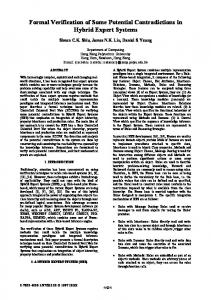
The source code of IRC is 600 lines of Coq functions and definitions. 1000 lines of Coq define generic data structures (and modules) that are not used directly by IRC. The whole proof represents approximately 4800 lines of Coq statements and proof scripts (excluding comments and blank lines), including 3300 lines (110 lemmas) for the properties of incremental update of worklists, 300 lines (17 lemmas) for the termination proof, 650 lines (22 lemmas) for the soundness proof and 550 lines (55 lemmas) for the properties of interference graphs. The proof is therefore 8 times bigger than the code it proves, which is a common ratio in the CompCert development [17]. We have integrated our IRC in the CompCert compiler. Thus, we can compare our Caml implementation of IRC (that is automatically generated from our Gallina program) with the Caml imperative one of CompCert. This comparison is done on the CompCert benchmark, whose characteristics are given in Fig. 4. The test programs range from 50 to 3000 lines of C code. Classically, for each program, the compiler generates at most two graphs for each function, one for integer variables and one for float variables. IRC is applied separately to each graph. Each line of Fig. 4 represents a program. The columns show the number of nonempty graphs to color, as well as the average numbers of vertices, interference edges and preference edges of these graphs. Integrating our IRC in the CompCert compiler allows us to compare the running times of both register allocations. The results on the CompCert benchmark are shown in Fig. 5. Measurements were performed on an Apple PowerMac workstation with two 2.0 GHz PowerPC 970 processors and 6Gb of RAM, running MacOS 10.4.11. The first two columns of the histogram show the running times of both allocators in milliseconds. Our allocator does not run as fast as the imperative one : a logarithmic penalty arising from operations on data structures 1 occurs. However, compilation times remain good (under 10 s. for all the programs of the suite); the slowdown is perfectly acceptable practically. 16
benchmark graphs variables interferences AES cipher 7 113 586 Almabench 10 53 310 Binary trees 6 23 42 2 50 332 Fannkuch FFT 4 72 391 Fibonacci 2 17 18 Integral 7 12 12 17 24 74 K-nucleotide Lists 5 18 33 Mandelbrot 2 45 117 N-body 9 28 73 2 25 53 Number sieve Number sieve bits 3 76 58 Quicksort 3 28 116 SHA1 hash 8 34 107 9 14 35 Spectral test Virtual machine 2 73 214 Arithmetic coding 37 31 85 32 127 Lempel-Ziv-Welch 32 Lempel-Ziv 33 29 92
preferences 166 22 14 27 37 9 5 14 11 17 10 12 12 16 15 6 38 15 16 15
Fig. 4. Benchmark characteristics.
The third column represents the virtual time obtained by adding a logarithmic penalty to the imperative allocator. In other words, the last column is (log n) times the running time of the imperative allocator, where n is the number of vertices of the graph. This virtual measurement emulates the penalty due to logarithmic-access to data structures. It enables a qualitative comparison between our functional IRC and a standard imperative implementation. The time spent by our allocator is very close to that of the imperative implementation with a logarithmic cost factor. Last but not least, we have compared the quality of executable code generated by both allocators. Actually, both allocators implement the same algorithm. We have measured the execution times of several executions of the test suite. The results are equivalent for each test case.
9
Related Work
Despite their wide use in computer science and the maturity of their theory, graphs are the subject of only a few works in the theorem-proving literature. Only a small part of graph theory has been represented in proof assistants. A few works on graphs are devoted to the specification of graph theory basics. In 1994, Chou formalized in HOL some usual notions of graph theory [11], e.g. graphs, digraphs, acyclic graphs, trees. Works of Chou were followed by formalizations of planar graphs [21] and of graph search algorithms [22] in HOL. In 17
Comparison of running times of the allocators (in milliseconds) 100
Imperative Caml allocator Functional formally verified allocator Imperative Caml allocator with (log N) penalty
90 80 70 60 50 40 30 20 10 0
ss lz w lz e d co ar h ac vm ral t ec sp a1 sh t or ts qs ebi v ie ns e v ie ns y od rot nb elb d an m ts ide lis leot uc kn r g te in
fib fft uch k nn es fa ytre r na ch bi ben a m al s
ae
Fig. 5. Comparison of the running times of our register allocator and the Caml one. To improve readability, results for the third column of almabench and fft are bounded by 100 though they are actually respectively 131 and 120.
2001, Duprat formalized the same notions as Chou and directed graphs in Coq, using inductive definitions. Unfortunately, these definitions cannot be extracted using the Coq mechanism for extraction. Hence our work does not use this library. Mizar is probably the theorem prover in which graph theory has been studied the most. It provides a large library on graphs including previous-cited basics and more elaborated formalizations as the one of chordal graphs. Other work naturally focuses on polynomial graph problems and their algorithms. More precisely, the most studied problem is the (very classical) problem of the shortest path in a positive-weighted graph. In 1998, Paulin and Filliˆ atre proved Floyd’s algorithm using Coq and a tool for verifying imperative programs that will become Caduceus later. To fit this tool, their algorithm is written in an imperative style where graphs are simply represented as matrices. Another algorithm for the same problem, Dijkstra’s algorithm, has been formalized and proved correct in both Mizar [10] and ACL2 [18]. Again, Mizar is in advance with the formalizations of other algorithms as the Ford-Fulkerson algorithm for flows, LexBFS for chordal graph recognition, or Prim’s algorithm for minimum spanning tree. The latter algorithm has also been proved correct using B [1]. Kempe proved the five-color theorem for planar graphs in 1879 using a variation of the simple algorithm described in the second paragraph of this paper. 18
Alas, he had no mechanical proof assistant; his “proof” of the four-color theorem [16] had an error that was not caught by mathematicians for 11 years. Appel and Haken proved the four-color theorem 97 years later [4]; this was the first use of a computer to prove a major open problem that was unsolved without mechanization. But major parts of that proof were unmechanized. Recently, the theoretical problems of reasoning about planar graph coloring have been tackled in modern proof assistants. Bauer and Nipkow formalized undirected planar graphs and discussed a proof of the five-color theorem in Isabelle/HOL [5]. Gonthier and Werner produced the first fully mechanized proof of the four-color theorem, using a formalization of hypergraphs which are a generalization of graphs [14]. Gonthier and Werner’s proof includes graph algorithms implemented in Gallina and reasoned about in Coq. Our work is significant for many reasons. It constitutes the first machinechecked proof of a nontrivial register allocation algorithm and a reference implementation of IRC. In addition, using a functional language, such as Gallina, and a recursive definition of an algorithm, requires hard work on the termination proof. Furthermore, the algorithm we prove is an optimizing algorithm working on interference graphs. These graphs have specific properties that must be kept in mind along the specification of the algorithm. Finally, we took a special care of the algorithmic complexity of the generated code since it deals with a real and concrete problem, register allocation that has been integrated to the CompCert compiler.
10
Conclusion
We have presented, formalized and implemented an optimizing register allocation algorithm based on graph coloring. The specification of this algorithm raises difficult programming issues, such as the proof of termination, the specification of interference graphs, the care of algorithmic complexity and the functional translation of an imperative algorithm. In particular, we provided a very accurate way to adjust worklists incrementally, even better than the ones usually implemented. We also provided a correct reference description of IRC. Technically, this work required the use of advanced features of the Coq system : mainly automatic generation of induction principles for non-structural recursive functions, but also dependent types for factoring development and proofs, generic modules, and efficient data structures. The automatic extraction of our implementation leads to a Caml code that has been embedded in CompCert and whose results are equivalent to the one of the current release version of CompCert. The execution times (of the graph coloring phase of the CompCert compiler) are competitive with the ones of the release version of CompCert. Only a very little slowdown that cannot be avoided appears, due to logarithmic data structures operations of purely functional programming. 19
References 1. Jean-Raymond Abrial, Dominique Cansell, and Dominique M´ery. Formal derivation of spanning tree algorithms. In ZB 2003, volume 2651 of LNCS, pages 627–628, 2003. 2. Andrew W. Appel. Modern Compiler Implementation in ML. Cambridge University Press, 1998. 3. Andrew W. Appel and Lal George. Optimal spilling for CISC machines with few registers. In PLDI, 2001. 4. Kenneth Appel and Wolfgang Haken. Every planar map is four colorable. Bulletin of the American Mathematical Society, 82:711–712, 1976. 5. Gertrud Bauer and Tobias Nipkow. The 5 colour theorem in Isabelle/Isar. In TPHOLs, volume 2410 of LNCS, pages 67–82, 2002. 6. Yves Bertot and Pierre Cast´eran. Interactive Theorem Proving and Program Development. Coq’Art: The Calculus of Inductive Constructions. Texts in Theoretical Computer Science. Springer Verlag, 2004. 7. Sandrine Blazy, Zaynah Dargaye, and Xavier Leroy. Formal verification of a C compiler front-end. In FM 2006, volume 4085 of LNCS, pages 460–475, 2006. 8. Preston Briggs, Keith D. Cooper, and Linda Torczon. Improvements to graph coloring register allocation. TOPLAS, 16(3):428 – 455, 1994. 9. Gregory J. Chaitin, Marc A. Auslander, Ashok K. Chandra, John Cocke, Martin E. Hopkins, and Peter W. Markstein. Register allocation via coloring. Computer Languages, 6:47–57, 1981. 10. Jing-Chao Chen. Dijkstra’s shortest path algorithm. Journal of Formalized Mathematics, 15, 2003. 11. Ching-Tsun Chou. A formal theory of undirected graphs in higher-order logic. In Workshop on Higher Order Logic Theorem Proving and Its Applications, pages 144–157, 1994. 12. Coq. The coq proof assistant, http://coq.inria.fr. 13. Lal George and Andrew W. Appel. Iterated register coalescing. TOPLAS, 18(3):300–324, 1996. 14. Georges Gonthier. Formal proof – the four-color theorem. Notices of the American Mathematical Society, 55(11):1382–1393, December 2008. 15. Sebastian Hack and Gerhard Goos. Copy coalescing by graph recoloring. In PLDI, 2008. 16. A. B. Kempe. On the geographical problem of the four colors. American Journal of Mathematics, 2:193–200, 1879. 17. Xavier Leroy. Formal certification of a compiler back-end or : Programming a compiler with a proof assistant. POPL, pages 42–54, 2006. 18. J. Strother Moore and Qiang Zhang. Proof pearl: Dijkstra’s shortest path algorithm verified with ACL2. In TPHOLs, volume 3603 of LNCS, pages 373–384, 2005. 19. George C. Necula. Translation validation for an optimizing compiler. SIGPLAN Not., 35(5):83–94, 2000. 20. Amir Pnueli, Michael Siegel, and Eli Singerman. Translation validation. In TACAS ’98, volume 1384 of Lecture Notes in Computer Science, pages 151–166, 1998. 21. Mitsuharu Yamamoto, Shin-ya Nishizaki, Masami Hagiya, and Yozo Toda. Formalization of planar graphs. In Workshop on Higher Order Logic Theorem Proving and Its Applications, pages 369–384, 1995. 22. Mitsuharu Yamamoto, Koichi Takahashi, Masami Hagiya, Shin-ya Nishizaki, and Tetsuo Tamai. Formalization of graph search algorithms and its applications. In TPHOLs, LNCS, pages 479–496, 1998.
20