Per Kristian Lehre, University of Birmingham, UK. [email protected]. Frank Neumann, Max Planck Institute for Infor
„hinking —fresh helpsF ƒurprisingly enoughD we ™—n develop — very f—st ....
QT. RW. TR c . c. c c c . c. c c m. m m. ¢¢¢ .fff m. m m. ¢¢¢ .fff m. 44444 .˜˜˜˜˜ m.
(Pearl 1988), statistics (Lauritzen 1996), and neural networks (Hertz,. Krogh, and Palmer ..... malism provides a more satisfactory framework in which to express this model. Moreover ... Redwood City, CA: Addiso~~-Wesley. Hinton, G. E., and ...
A "graphical model" is a type of probabilistic network that has roots in several different research communities, including artificial intelligence. (Pearl 1988) ...
then ten years to develop the foundation of this paper since. Proceedings of the .... numbers in the Ada programming language [Barnes 1989,. 1992, 1995, Watt ...
Dec 12, 2013 - Abstract Turing machines and Gödel numbers are important pillars of the ...... Hofstadter, D.R.: Gödel, Escher, Bach: an Eternal Golden Braid.
Dec 12, 2013 - Turing computation in a neural field environment. To this end, we employ .... functions that are not admitted for the dynamical law (3). Therefore, vari- ables have to be ...... 2012 - Alan Turing 2012, vol. 5th AISB Symposium on ...
A series of load tests on jacked tubular piles are reported. These tests ... Previous testing of pressed-in pile foundations is reported by White et al (2003). A series ...
Dec 11, 2015 - We developed a numerical method to compute the gravitational field ... vector by numerically differentiating the potential by Ridders' algorithm.
electronic components. The demands for volume, weight and cost reduction foster a compact and ... Canonical Cauer networks can describe radiation modes. The lumped element ... a proper definition of integral field quantities. One particular .... form
and contains only interconnects, including ideal transformers. ..... lumped element circuit represented by a network, the spatial subdomains may be considered ...
May 21, 2004 - INSTITUTE OF PHYSICS PUBLISHING ... Efficient computation of lead field bases and influence ... algorithms for their efficient computation.
Jul 25, 2017 - We developed a numerical method to compute the electromagnetic ... by numerically differentiating the numerically integrated potentials by the ...
May 29, 2016 - Key words: gravitation â celestial mechanics â protoplanetary discs â methods: numerical. â galaxies: general .... these basic density functions, this approach seems sufficient. ...... In order to avoid this problem, Danby (198
Computation of Three-Dimensional. Electromagnetic Field Including Moving Media by. Indirect Boundary Integral Equation Method. Dong-Hun Kim, Song-Yop ...
This paper addresses the problem of mobile robot navigation using artificial potential fields. Many potential field based methodologies are found in the robotics ...
non-linear distance function of each primitive as a dot prod- uct of linear factors. ... Main Results: In this paper, we present a new algorithm ..... The separation angle criterion acts like a low-pass filter and is ... As the grid resolution increa
Department of Computer Science ... compute 3D distance fields of complex models at interactive .... The underlying distance function is a degree two function.
Nov 25, 1992 - arXiv:hep-th/9211100v2 25 Nov 1992. November, 1992 ..... Indeed, this is exactly the correct number of the primary fields as defined by eq. (6).
Mar 25, 2004 - From these postulates we will obtain rigorous and general proofs that ... relativistic field theory, such as CPT and spin-statistics theorems, ...
At the 0th clock tick, NS1 and NS2 are 0. For all further clock ticks, the outputs of the neurons are NS1 and NS2 (for neuron 1 and 2 respectively). c) EXS is the ...
Schunck [3] uses clustering of local gradient-based constraints and surface-based smoothing. Odobez and. Bouthemy [4] use an M-estimator based on an affine.
evidence so gained raises interesting questions about the best possible decay rates ...... computer. The computer is a Lenovo T61p laptop with a dual core 2.4 ...
Many simulators, including most digital circuit simu- lators, are based on a ..... and the following com- panies: Bell Northern Research, Cadence, Dolby, Hitachi,.
Foundations of Field Computation Bruce MacLennan Copyright c 2012 Draft of August 31, 2012
Chapter 4 Basic Complex Analysis Although real numbers are sufficient for most applications of field computation, complex numbers are sometimes required, as in Fourier analysis and the application of field computation is in quantum computation. Therefore the goal of this chapter is to provide an intuitive understanding of basic complex analysis, especially as it applies in Hilbert spaces; a systematic presentation of complex analysis is beyond its scope. In addition to standard material, this chapter includes a brief discussion of hyperbolic trigonometry and its applications in special relativity theory, which is intended to build intuition by stressing the analogies with ordinary (circular) trigonometry.
4.1
Argand diagram
p As everyone knows, complex numbers involve i = 1. However, it will be p better at this point to forget about 1 and understand complex numbers by means of the Argand diagram (Fig. 4.1). As a matter of history, mathematicians were dubious about imaginary numbers, and questioned their legitimacy, until familiarity with the Argand diagram showed that they could be thought of as ordinary two-dimensional vectors. For in the Argand diagram we simply represent the complex number x + iy as a vector (x, y). (In this sense “i” can be thought of as a place holder or tag to distinguish the Y-coordinate from the X-coordinate.) Then operations on complex numbers can be interpreted as operations on two-dimensional vectors, without conp cern for 1. When complex numbers are represented in this way, they are said to lie in the complex plane. Real numbers lie along the positive and 41
42
CHAPTER 4. BASIC COMPLEX ANALYSIS Im
z
y r q
x
Re
Figure 4.1: Argand diagram. z = x + iy = rei✓ .
negative X-axis, and (pure) imaginary numbers along the positive and negative Y-axis; other points represent complex numbers with both (nonzero) real and imaginary parts. Therefore, in the complex plan the X-axis is called the real axis and the Y-axis is called the imaginary axis. (Why we should bother with complex numbers, and not simply make do with two-dimensional vectors, will become apparent as we proceed.) Remark 4.1.1 Notice that, unlike the real numbers, there is no natural sense in which the complex numbers can be ordered. Definition 4.1.1 (Cartesian components) The < : C ! R and = : C ! R operators extract the Cartesian components (real and imaginary parts, respectively) of a complex number: