FPGA Implementation of QCWT Based Algorithm for Filtering Low SNR Signals A. Marcianesi, R. Padovani, N. Speciale, N. Testoni, G. Masetti DEIS University of Bologna Viale Risorgimento 2, 40136 Bologna, ITALY email:
[email protected]
ABSTRACT In this work we present and validate a new algorithm suitable for detecting, filtering and restoring Sonar pulses in presence of strong noise, and Doppler frequency shift. The algorithm: i) is based on the Quasi-Continuous Wavelet Transform (QCWT) and enables to get very good matching between transmitted and received signals also for low signal-tonoise ratio; ii) exploits the high time-scale resolution offered by considering octave and sub-octave division schemes, and iii) allows both an easy hardware FPGA implementation and real time processing capabilities and, thus, is particularly suited for biomedical applications and material properties investigations. 1
Introduction
In order to reduce the presence of noise, digital signal processing of sonic and ultrasonic waveforms requires the use of advanced denoising filtering. This is particularly true for spectral images of biological tissues as well as vector images of blood flow; in some applications such as biomedical tissue microstructure reconstruction, material properties investigations or microwave automotive radar systems, the received echoes are so strongly corrupted by interfering signals that the system is not able to extract the information [6][7][8]. Moreover, the design of automatic signal detection or recognition systems represents a formidable challenge to the processor tasked to extract distinguishable features for classification or denoising because of the presence of weak signals related to surrounding noise, so it is mandatory a reliable method to recover the objects’ echoes. To extract important non-stationary real signal characteristics such as drift, trends and abrupt changes, classical methodologies like pass-band filtering, FFT based processing or spread-spectrum techniques cannot be effective or suitable for real time applications.
On the contrary, the multiresolution properties of the Wavelet Transform can reveal the time evolution of the spectrum, as the signal analysis is performed in a time-frequency domain. As well known, the Continuous Wavelet Transform (CWT) [1][2] is defined as the orthogonal projection of the signal x(t) ∈ L2 (R) on the functional space defined by the functions ga,b (t): CW T (x, g; a, b) = hx|ga,b i where a ∈ R+ \ {0} is the scale or dilatation parameter and b ∈ R is the time or translation parameter. Though the CWT redundancy allows to operate at every scales, for computational reasons different sampling methods have been applied to the domain of the dilation and translation parameters, so different wavelet transformation techniques can be introduced to improve time-frequency resolution or computational efficiency. For the Discrete Wavelet Transform (DWT) the scale and time parameters are defined respectively as a = 2j and b = k where j, k ∈ N: the result is a very fast implementation [2] that does not introduce any form of redundancy but has a very poor timescale resolution at the higher scales, introducing an upper limit in the scale domain. The Stationary Wavelet Transform (SWT) tries to avoid the poor time-scale resolution keeping a low computational cost by defining the scale and time parameters respectively as a = 2j and b = k where j, k ∈ N; an efficient implementation of this technique consists in a filter bank where each filter is the dyadic up-sampled version of the previous one. Finally, the Quasi-Continuous Wavelet Transform (QCWT) is an even better solution to the poor timescale resolution of the DWT but it is computationally heavier than the SWT [3]. Scale and time parameters are defined as a ∈ R+ \ {0} and b ∈ N: this means that only the time parameter has been sampled, while the scale parameter can be set ac-
cording to the design constraints. As the SWT, an efficient implementation of the QCWT uses a filter bank but direct relations between filters cannot be always shown. For our applications, we investigated all the previous described methods and defined suitable filtering structures to implement them in hardware. 2
Description of the proposed algorithm
The four steps of the proposed algorithm are as follows. In the first one we compute the WT of the received signal which samples are used to calculate the coefficients of the wavelet expansion. This step is implemented with a convolution operator corresponding to an optimized FIR filter with different tap coefficients according to the type of wavelet transform chosen. As a second step, a pattern matching procedure is applied on the data stream to find the coefficients more similar to those obtained from the corresponding wavelet transformation of the ideal pulse profile. Data denoising was done by removing the coefficients according to the pattern matching procedure. Finally, the inverse CWT is computed according to the transformation chosen in the first step. By so doing, we get the time profile of the received signal, filtered from noise and jamming, together with the informations related to the Doppler shift. 2.1 Wavelet Analysis For the DWT the definition of the algorithm for the calculus makes use of approximation coefficients, resulting from the projection of the signal x(t) on the functional space generated by the family of functions fj,k (t), and detail coefficients that result from projection of the signal on the functional space generated by the functions gj,k (t): A0,k (t) Aj,k
=
Z
+∞
x(t)F (t − k)dt
approximation and the detail channel respectively and a dyadic down-sampler that operates only on the approximation channel; each stage takes its inputs from the previous stage approximation output channel. Despite the SWT may resembles the DWT, it is worth noting that its complexity grows exponentially with the number of octaves. The algorithm used for the calculus of the SWT can be defined as: Z +∞ x(t)F (t − k)dt A0,k (t) = −∞ X L2−(j−1) (n−k) Aj−1,n Aj,k = n
Dj,k
=
X
Ln−2k Aj−1,n
=
X
Hn−2k Aj−1,n
H2−(j−1) (n−k) Aj−1,n
n
The SWT has the same structure of the DWT [2] as each hardware stage implements an octave and is composed by two FIR filters respectively for the approximation and the detail channel; however in this case the filters coefficients are not constant through the whole system: in fact at each stage an exponentially growing number of zeros are inserted between the elements of Lk and Hk . Conversely, the QCWT uses a totally different approach to overcome the poor time-scale resolution of the DWT [3]. It uses a filter bank where filters are independent from one another and each one is used to compute a single scale; moreover, there are no approximation channels as each stage directly gives the wavelet coefficients. Since only the time parameter is sampled, this is very useful in digital system, where the data channel does not bear a timecontinuous information but is a sampled version of a time-continuous signal. Whenever the scaling function f (t) is orthogonal to its integer translations, it is possible to calculate the coefficients of the used filter qa [n]:
−∞
=
X
qa [n] =
ha−1/2 g(a−1 t)|f (t − n)i hf (t)|f (t)i
(1)
n
Dj,k
n
where Aj,k (t) and Dj,k (t) represent the approximation and detail coefficients respectively; Lk = 2−1/2 ck and Hk = 2−1/2 dk are the FIR filter coefficients, while F (·) is a suitable pre-filtering function. The scale parameter j defines the octave at which the transform is computed; each hardware stage implements an octave and is composed by two FIR filters with coefficients Lk and Hk respectively for the
so the QCWT algorithm is defined as: X Da,b = A0,n · qa [n − b] n
A0,n
=
Z
+∞
x(t)F (t − b)dt −∞
where g(t) is the wavelet function. It is quite simple to build a system based on the QCWT algorithm: in fact the whole system consists of a bank of filters whose coefficients can be precalculated through
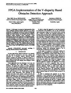
Figure 1: QCWT Architectural View. From the top-left to the bottom-right: the common term multiplier, the chain of auto-zeroing registers forming the memory stage of the filter, the bank of shifters/sign extender needed to implement the power-two multiplications, the bank of multipliers that implements the filter coefficients and finally the adder tree needed to generate the final outcome of each filter. eq. (1) Fig. 1 shows the implemented architecture solution for the QCWT algorithm. In particular, the Haar wavelet implements an optimized version of the standard QCWT algorithm scheme by using a parametric representation for the scale paramem+nM ter a = 2 M to obtain sub-octave filtering, where M ∈ N is the number of sub-octave for any octave, m ∈ [0, M − 1] ⊂ N is the sub-octave coordinate and n ∈ N is the octave coordinate. By so doing we get to an optimized filter definition that needs at most only three multiplications: two for each filter and one common to the corresponding sub-octaves defined only by m ∈ [0, M − 1]. Such an optimized structure is represented in
Fig. 1 for the dual corresponding sub-octave filter case, where we use the following parameters: M = 4, m = 1, n = {1, 3}, leads to a strong reduction in chip area occupation. Each multiplier uses two clocks and implements a serial algorithm: software simulations showed that this unit can operate at a maximum clock speed of 38.6MHz on the EPF10K20RC240 chip, using only 55 LCs when the multiplier is assigned and constant. Therefore, as the same FPGA supports ripple-carry adders with I/O delay of 6.3ns, the highest system clock frequency (given by the multipliers clock speed divided by the number of iterations in the serial multiply algorithm) is approximatively 2.4MHz.
Software simulations and hardware results for the first sub-octave/first octave (1.1) and for the first sub-octave/third octave (3.1) show an absolute HW error limited to ±LSB i.e. ±0.244 · 10−3 for a 12 bit system and ±3.906 · 10−3 for an 8 bit system. 2.2
max_pattern_load min_pattern_load low_threshold_load high_threshold_load
max/min
dv
pfo
max
stream
data_in
min
threshold
comparison
dv
dvo mko
Pattern matching and denoising load
The purpose of the second stage is to recognize and extract the presence of a specific signal pattern in the wavelet spectrum passed as input. Since pattern matching is an extremely complex operation in its most general form, the solution discussed here is actually a specialized one, which has been simplified to allow for an efficient implementation and which is applicable to a limited, though very large, subset of possible input signals. All of the signals of interest show a common general behaviour when viewed in the wavelet domain: at a given scale, the typical shape shows a swing between a maximum and a minimum value. Only single-scale analysis was taken into account: at a given scale, the typical shape shows a swing between a maximum and a minimum value. Thus, the idea behind the algorithm is that the recognition of a particular signal is possible by searching for its known pattern maxi-min-max sequences. The whole process is split into two sequential tasks: the isolation of the max/min scheme and the comparison between the collected data and those we are looking for. Both of these tasks were defined for an efficient FPGA implementation, avoiding both the use of loops (i.e. datapath-control unit) and the storage of the whole signal (i.e. huge quantity of memory). We defined a streaming process since operating on the flow of the signal requires virtually no memorization of it and does not need to loop around a set of data. Maximum and minimum values extraction is coupled with an inner step to perform a thresholding operation, so that most of the noisy peaks will not proceed to the following elaboration steps where they might increase the chances of a false revelation. Moreover, the relative distance between peaks was compared with the expected one, and the boolean value at the output states if the pattern is present or not. Additionally, to overcome possible distortion and Doppler effects the signal may have undergone before processing, a user-defined tolerance was considered when comparing the distances. The first block in Fig. 2 searches for all of the maximum and minimum values of the signal: in particular, it implements a finite state machine that keeps
Figure 2: Architectural view of the pattern matching stage and I/O signals. The figure shows the data in signal through which data are synchronously fed into the block, the programming buses together with their load command, which control the threshold level applied and the max/min pattern.
Figure 3: Example of pattern matching procedure. track of the positive or negative slope and that forwards to the output stream only values corresponding to a change in the derivative. By so doing, we get a very efficient elaboration and a low area occupation in terms of logic cells required on the FPGA. After thresholding, the last block performs the comparison: the signal is windowed and logically combined with the pattern to produce a boolean output (pfo in Fig. 3), synchronous with the analyzed signal, stating whether a pattern has occured or not. As we can see in Fig. 3, the signal pfo is high when a pattern is found in the input signal data in, according to the pattern loaded in the two registers max pattern load and min pattern load. 2.3
Inverse Wavelet Synthesis
According to the transformation chosen, as a final step, we computed the wavelet reconstruction. We assumed that the approximation coefficients at the higher scale are zero, together with the detail coefficients at the lower scales not meaningful for the processing. As a result, we obtain the time profile of the received signal filtered from noise and jamming
for typical Radar/Sonar applications. The methodology has been successfully applied to detect and reconstruct real Sonar pulses obtaining almost perfect matching between the transmitted and the received signals up to a SNR level of -5dB.
Comparison between Hardware and Matlab outputs 1
0.8
0.6
Amplitude
0.4
References
0.2
0
[1] I. Daubechies, “Ten Lectures on Wavelets” CBMS-NSF Regional Conference Series, SIAM, Philadelphia, 1992.
−0.2
−0.4
−0.6
−0.8
−1
0
200
400
600
800
1000
1200
1400
1600
1800
2000
Time samples
Figure 4: Comparison between Matlab cients at scale 32 and the measured ones.
TM
coeffi-
signals, maintaining good information related to the Doppler shift in frequency. 3
Results
The proposed algorithm was tested with both synthetic test and physical signals representing simple but typical sonar applications. The synthetic input signals were corrupted by white noise to test filter sensitivity. Random noise, with a Gaussian density function, was generated by MatlabT M [9], and the noise variance was related to the l 2 norm of the signal to obtain different signal-to-noise ratio. As an example, to simulate the first block we use a synthetic signal si , a sinusoidal burst with 3 cycles corrupted by AWGN with σ = 0.5. Fig. 4 shows the comparison between the wavelet coefficients at scale 32 as computed by Matlab (line), and the FPGA 8-bit output sampled by the oscilloscope (dots). Finally, Fig. 3 shows an example of the second stage output in the pattern matching stage: the presence of a correct max-min-max pattern sequence is recognized in the test signal data-in. 4
Conclusions
In this work we presented a new flexible QCWT wavelet-based algorithm that is able to correctly recognize a specific pattern in a noisy signal, to filter signals with a very low SNR. The careful area optimization makes it possible for the implementation to fit on a single FPGA chip (where number of connections, memory and logic cells are considerable constraints) with the speed and accuracy required
[2] O. Rioul, P. Duhamel, Fast Algorithms for Discrete and Continuous Wavelet Transforms in IEEE Trans. Inform. Theory, vol. 38, pp. 569586, March 1992 [3] S. H. Maes, Fast Quasi-Continuous Wavelet Algorithms for Analysis and Synthesis of onedimensional signals in SIAM J. Appl. Math., vol. 57, pp. 1763-1801, Dec. 1997 [4] A. Marcianesi, S. Scaletti and N. Speciale “A Wavelet-Based Algorithm for Filtering Radar/Sonar Signals with Low Signal-to-Noise Ratio” Proc. NSIP 2001 June 3-6 Baltimora, Maryland USA. [5] C.K. Chui, “An introduction to Wavelets,”, Academic Press, San Diego, 1992. [6] E. Elsehely and M.I. Sobhy, “Detection of Radar Target Pulse in the Presence of Noise and Jamming Signal using the Multiscale Wavelet Transform,” Proc. of ISCAS ’99, Vol.3, pp. 536-539 1999. [7] B. Liu, Y. Wang, W. Wang, “Spectrogram enhancement algorithm: a soft thresholding based approach,”, Ultrasound in Med. and Biol., Vol. 25, n. 5, pp. 839-846, 1999. [8] W. Chen, G. Zhou, G.B. Giannakis, “Velocity and acceleration estimation of Doppler weather radar/lidar signals in colored noise,”, Proc. of ICASSP95, Vol. 3, pp. 2052-2055, 1995. [9] “Matlab Reference Manual”, The Math Works Inc. [10] Y. Mayer, Ondelettes et oprateurs I: Ondelettes, Hermann, Paris, 1990