From Markov Random Fields to Associative Memories and ... - CiteSeerX

From Markov Random Fields to Associative Memories and Back: Spin-Glass Markov Random Fields B. Caputo, H. Niemann Computer Science Department, Chair for Pattern Recognition, University of Erlangen-Nuremberg, Martensstrasse 3, D-91058, Erlangen, Germany Phone +49 9131 8527824; fax: +49 9131 303811 E-Mail: {caputo, niemann}@informatik.uni-erlangen.de In this paper we propose a fully connected energy function for Markov Random Field (MRF) modeling which is inspired by Spin-Glass Theory (SGT). Two major tasks in MRF modeling are how to define the neighborhood system for irregular sites and how to choose the energy function for a proper encoding of constraints. The proposed energy function offers two major advantages that makes it possible to avoid MRF modeling problems in the case of irregular sites. First, full connectivity makes the neighborhood definition irrelevant, and second, the energy function is defined independently of the considered application. A basic assumption in SGT is the infinite dimension of the configuration space in which the energy is defined; the choice of a particular energy function, which depends on the scalar product between configurations, allows us to use a kernel function in the energy formulation; this solves the problem of high dimensionality and makes it possible to use SGT results in an MRF framework. We call this new model Spin Glass- Markov Random Field (SG-MRF). Experiments on textures and objects database show the correctness and effectiveness of the proposed model.

1 Introduction In the last few years there has been a growing interest within the computer vision and machine learning community in Spin Glass Theory (SGT) [15] and its possible application in learning and recognition tasks. SGT was first used in physics to describe magnetic materials in which the interactions between the magnetic moments (spins) are random and conflicting. The attempt to understand the cooperative behavior of such systems has led to the development of new concepts and techniques which have been finding applications and extensions in many areas such as 1

attractor neural networks [1], combinatorial optimization problem [15] and prebiotic evolution [15]. The reason why the idea to extend SGT results in different contexts is so appealing is that SG is, until now, the only model of a disordered system which is fully understood from a theoretical point of view. Physicist have studied for a long time disordered systems trying to find a hidden order; in recent years they have discovered that the collective behavior of a disordered macro-system, i.e. a system composed of many entities (for instance magnetic materials and spins), does not change qualitatively when the behavior of single components are modified slightly. There are universal classes which describe the collective behavior of the system, and each class has its own characteristic; moreover, the universal classes do not change when we perturb the system. From the point of view of computer vision, the macro-system and the entities can be an image and its pixels; an object and the features which describe it; a scene and the different objects which compose it and so on. In all these examples, the components can be modeled as random variables, and they interact between each other in a sometimes cooperative, sometimes conflicting way; all these interactions give rise to a collective behavior which is the macro-system. Some approaches have already been proposed in order to integrate SGT results in suitable framework for computer vision and machine learning: the first attempt was done by Parisi [15] which modeled a matching problem with SG mathematical tools; more recently Opper proposed a SG approach to Gaussian Processing, first using a naive mean field approximation [18] and more recently using a replica method approach [14]; Amit and Mascaro [2] proposed an attractor neural network composed by thousands of binary perceptrons which successfully recognize shapes, in context with a very large number of classes. Perceptrons have randomized feed forward connections, modified using field dependent Hebbian learning; each class is represented by a pre-learned attractor, which acts as an associative ‘hook’. In this paper we propose Markov Random Fields (MRF) [12] theory as the natural framework for integrating SGT results for computer vision applications. The mathematical formulation of equilibrium statistical mechanics is the same as for MRF models; as a consequence of full connectivity (which is a main feature of SG models), the Markovian property is automatically satisfied; the conclusion is that a SG model is a MRF model. Another very strong motivation for integrating SG results in a MRF framework is that it makes it possible to apply MRF on classes of problems on which until now its application has been so difficult to make it almost impossible. A MRF is defined with respect to a given neighborhood system, given an energy function which properly models the constraints between them. The neighbor relations between sites is defined respect to their regularity; in the case of regular sites the definition is generally straightforward, and many successful applications can be found in literature (see for instance the monographs [26, 12]). It is important to note that approaches which use MRF based models solve mostly low level image processing problems [27, 26]. Only a few authors consider the high level vision task of object recognition using MRF [25, 13, 16]. This is due to the fact that high level vision tasks have to be generally modeled by irregular neighborhood systems, 2

which are mostly defined by means of heuristic distances, generally feature-dependent. Consider for instance 3D object recognition as application problem: if the chosen features are not invariant to pose (as it is often the case), pose parameters should be incorporated into the energy formulation and in the neighbor relations definition, with a dramatic increase in complexity; furthermore, due to mutual occlusion, neighborhoods change with pose parameters. Regarding the energy function, in the case of irregular sites its formulation can become something of an art, as it is generally done manually. The problem of the neighborhood definition can be avoided in a fully connected MRF: full connectivity eliminates the need to define distances between sites, but it does not solve the problem of increased complexity; on the contrary, it increases it; see for instance Zhu [28], where a fully connected MRF is proposed for texture modeling: the MRF vocabulary results enriched, but the computational times are very high. SGT provides a way to deal with these problems in an elegant manner: full connectivity makes the neighborhood definition irrelevant, and the energy function is defined independently from the considered application; this makes it possible to find the analytical properties of the minima and may make it unnecessary to construct fast algorithms for searching the absolute minima. To our knowledge, there are no previous works attempting to integrate SGT results in a MRF framework. A basic assumption in SGT is the infinite dimension of the configuration space where the energy lives [15]. This condition cannot be satisfied for a generic pattern recognition problem, due to the curse of dimensionality [3]. The choice of a particular energy, which is a function of the scalar product between configurations [9, 1], allows us to use a kernel function [24, 20] in the energy formulation; this solves the problem of the high dimensionality and makes it possible to use SGT results for MRF modeling purposes: we call this new model Spin Glass-Markov Random Field (SG-MRF). The paper is organized as follows: in Section 2 we review the basic definitions of MRF theory, underlying the modeling problems in the case of irregular neighborhood systems. Section 3 introduces the basic ideas of SGT: as the topic is huge, we present here the main concepts and results in a context more familiar to the reader (hopefully); a detailed discussion on SGT and applications to attractor neural networks can be found in [15, 1]; more emphasis on the mathematical formulation and theoretical results is used in the description of the particular model for the energy function (Hebbian associative memory, [9, 1]) that we will use in the MRF model (Section 3.2). Section 4 presents SG-MRF: we show that the chosen energy can be written as a function of the scalar product between configurations; this opens the possibility of using kernel methods [20] in order to satisfy the basic requirement of equilibrium statistical mechanics, a high dimension (possibly infinite) of the configuration space. Indeed, the kernel trick maps the data in a higher, possibly infinite, dimensional space with respect to the space where the data lives [20, 24]. The consequences of the kernelization of the energy are unexpected and fascinating. The kind of kernel to be used must be chosen in order to satisfy theoretical constraints on the Hebbian energy, and those constraints lead to the choice of generalized Gaussian kernels [20] (Section 4.2). This choice makes it possible to interpret SG-MRF as a kernel3

ized Parzen windows [7] (Section 4.3); it also induces a histogram-based representation as the “natural” choice for the representation step; this makes it possible to interpret SG-MRF as a kernelized generalization of the FRAME model [28] (Section 4.4). Section 5 reports experiments performed using multidimensional receptive fields histograms [19] for the representation step; classification results are reported for textures and 3D objects. The results obtained with SG-MRF are compared with those obtained with a Nearest Neighbor Classifier (NNC) and a chi-square distance measure commonly employed in literature for histogram comparisons. For both experiments, SG-MRF gives the best performance. The paper concludes with a summary and possible future directions of research.

2 Markov Random Fields Markov Random Field (MRF) [26, 12] is a branch of probability theory which provides a foundation for modeling spatial interactions on lattice systems or, more generally, of interacting features. Labeling is a natural representation for the study of MRFs; furthermore, many vision problems can be posed as labeling problems in which the solution to is a set of labels assigned to image pixels or features. A labeling problem is specified in terms of a set of sites and a set of labels. Let S = {1, . . . , m} index a discrete set of m sites, and let L be a set of continuous (Lc = ℜa×b×... , (a, b, . . .) dimensions) or discrete (Ld = {1, . . . , M}, M number of labels) labels; the labeling problem is to assign a label from the label set L to each of the sites in S. The set f = {f1 , . . . , fm } is called a labeling of the sites in S in terms of the labels in L. When each site is assigned a unique label, fi = f (i) can be regarded as a function with domain S and image L. In the terminology of random fields, a labeling is called a configuration. The sites in S are related to one another via a neighborhood system. A neighborhood system for S is defined as N = {Ni |∀i ∈ S} : i ∈ / Ni , i ∈ Nt ⇐⇒ t ∈ Ni

(1)

where Ni is the set of sites neighboring i. A subset c of S is called a clique if two different elements of c are always neighbors. The set of cliques will be denoted by C. Let F = {F1 , . . . , Fm } be a family of random variables defined on the set S, in which each random variable Fi takes a value fi in L. For a discrete label set L, the probability that random variable Fi takes the value fi is denoted P (Fi = fi ), and the joint probability is denoted P (F = f ) = P (F1 = f1 , . . . , Fm = fm ). F is defined as a MRF on S with respect to a neighborhood system N if P (fi|fS−{i} ) = P (fi|fNi ), where S − {i} is the set difference, fS−{i} denotes the set of labels at the sites in S − {i} and fNi = {fi′ |i′ ∈ Ni }stands for the set of labels at the sites neighboring i. Note that every random field is a MRF when all different sites are neighbors. 4

A set of random variables F is said to be a Gibbs Random Field (GRF) on S with respect to N if its configurations obeys a Gibbs distribution: 1 1 P (f ) = exp − E(f ) , Z T 



Z=

X

{f }

1 exp − E(f ) . T 



(2)

The normalizing constant Z is called partition function, T is a constant called temperature, and E(f ) is the energy function. The energy E(f ) =

X

Vc (f )

c∈C

is a sum of clique potentials Vc (f ) over all possible cliques C. The value of Vc (f ) depends on the local configuration on the clique c. The Hammersley-Clifford theorem establishes the equivalence between MRF and the Gibbs distribution ([26, 12]): for a given Ni , P (f ) is a MRF distribution if and only if P (f ) is a Gibbs distribution. Two major tasks when modeling MRFs are how to define the neighborhood system for irregular sites, and how to choose the energy function for a proper encoding of constraints. The neighbor relations between sites is related to their regularity; in the irregular case [12], the neighborhood system is mostly defined by means of a heuristic distance that is featuredependent. The energy function is a quantitative cost measure of the quality of a solution, where the best solution is the minimum. In the case of irregular sites, the energy function’s formulation can become something of an art, as it is generally done manually. These problems are so relevant that until now MRF models have rarely been applied to computer vision tasks such as 3D object recognition, which should generally be modeled with irregular sites. The problem of the neighborhood definition can be avoided in a fully connected MRF: full connectivity eliminates the need to define distances between sites, but it dramatically increases the algorithm complexity.

3 Spin Glass Theory and Beyond 3.1 Spin Glasses The expression Spin Glasses (SG) was introduced to describe magnetic materials in which the interactions between the spins are random and conflicting [15]. The study of such systems has led to the development of a mean field theory of SG which have been finding applications and extensions in many areas such as attractor neural networks [1], combinatorial optimization problems, prebiotic evolution, and so on [15]. Two basic properties of SG are quenched disorder and frustration: quenched disorder refers to constrained disorder in interactions between

5

spins and/or their locations; frustration refers to conflicts between interactions, or other spin-ordering forces, such that all can be obeyed simultaneously. The relevance of frustration is that it leads to degeneracy or multiplicity of compromises. Here we are mostly interested in the mathematical structures arising from the study of SGs. Thus, we will introduce the reader to the essential ingredients of SG behavior describing some more familiar situations which can be mathematically modeled as SGs; a SG-like system will be described later. Life is often source of frustration: we usually have goals that are mutually incompatible, and we must give up some of them; this makes us feel frustrated. The situation is more complex when many people are involved; in Shakespeare’s tragedy such situations are very frequent [15]. Consider for example “Romeo and Juliet” [21]: there is a fight between two families, and all characters on the scene have personal relations to each other; some are friends and some are enemies. Assume for simplicity that all feelings are reciprocal, 1 and consider three characters: A, B and C. If A and B, B and C, and C and A have good relations there is no problem and they will be on the same side (this is the case for example of Juliet, Tybald and the Nurse). If A is friend of B, and C is an enemy of both A and B, A and B will be on the same side and C will be on the other side (for example Romeo, Mercutio and Tybald). If however, A and B and B and C are friends but A and C hate each other, someone must stay on the opposite side of his friend, a frustrating situation (for example Romeo, Juliet and Tybald). This analysis can be formalized by assigning to each pair (A and B) a number (JAB ) which is +1 if A and B are friends, and −1 if they are enemies. The relations between three characters (A, B and C) are frustrated if JAB · JAC · JCB = −1 When the relations of many triplets are frustrated, the situation on the scene is unstable and many rearrangements of the division in two sides are possible. These ideas can be formalized mathematically [15]: we have N variables si , one for each character; si takes values +1 or −1 depending on which side the i-th character stays, and for a given set of the Jij we are interested in minimizing the energy function E=−

X

Jij si sj

i, j = 1, . . . N.

(3)

(i,j)

The dynamic without errors corresponds to examining si sequentially and to set the si at the next step equal to [1] si (t + 1) = sign(hi (t)),

hi (t) =

N X

Jij sj (t),

∀i = 1, . . . , N.

(4)

j=1

If we want to introduce errors in the optimization process, the most elegant way consist in substituting (4) with [1] si = 1 1

with probability

p+ (hi );

If it is not the case, the system may never reach equilibrium [15].

6

si = −1

with probability

p− (hi ),

where hi is defined as in eq. (4) and the functions p+ (hi ) and p− (hi ) are given by [1] exp(βhi ) ; exp(βhi ) + exp(−βhi ) exp(−βhi ) p− (hi ) = . exp(βhi ) + exp(−βhi )

p+ (hi ) =

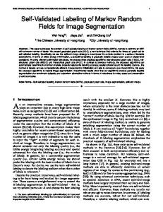
This way of introducing errors has the advantage that we can compute the probability distribution of the configurations of the {si }, i = 1, . . . , N at equilibrium. In that case we know that [1] X 1 PJ (s) = exp(−βE(s)); Z= exp(−βE(s)), (5) Z {s} which is formally identical to equation (2). In statistical mechanics eq. (5) is the Gibbs probability distribution and β is given by 1/KT , where K is the Boltzmann constant and T is the absolute temperature [1]. Many different dynamics can lead to the probability distribution (5); eq. (5) can also be considered as a way to weighting the configurations which are not optimal. For β → ∞ the probability distribution is concentrated on the optimal solution, while for large but finite β the probability distribution is concentrated on the nearly optimal configurations [1]. Different choices of the connection matrix J = [Jij ], (i, j) = 1, . . . , N will lead to systems with very different behaviors. In order to see this, let us consider four spins si which can assume values ±1, and which are placed at the four corners of a square; the lines connecting the spins indicates which spins are interacting to each other [1]. The energy of a given configuration of spins (s1 , s2 , s3 , s4 ) is given by (3), where the sum is over all pairs which are connected by lines in Figure 1. Jij will assume here values ±1: a positive (negative) sign indicates that two neighboring spins prefer to have the same (opposite) sign. In this example Jij = J = +1 (Figure 1, left). Every pair of spins on an edge would lower the energy by having the product of its values equal to the sign of the corresponding Jij . It is easy to verify that there are two configurations for which it is possible to arrange all four spins so that every single pair is ‘happy’ [1] (as to say, Jij si sj = 1 > 0); those configurations are S1 = S2 = S3 = S4 = +1, S1 = S2 = S3 = S4 = −1. For these configurations, eq. (3) will reach its lowest possible value (E = −4). Note that the two equilibrium configuration are equivalent under a symmetry transformation 2 . 2

For N → ∞ this is a 2D Ising model [1].

7

Figure 1: Two simple examples of Ising-like (left, (a)) and SG-like (right, (b)) systems. The system (a) does not present frustration, the system (b) does. Consider now a different choice for the value of Jij ( Figure 1, right): J12 = J23 = J34 = +1, J14 = −1. It is easy to see that now there is no configuration of the four spins which can satisfy all four bounds: the bound 1 − 4 would like its two spins to be of opposite signs, but all other bounds would like to align 1 with 2, 2 with 3 and 3 with 4. These three bounds would tend finally to align 1 and 4, leading to a contradiction. There is, therefore, no configuration which can give an energy as low as −4. Thus, the system is frustrated. The lowest energy value for this system is E = −2, and there are 8 configurations of lowest energy: S1 = S2 = S3 = S4 = −1; S1 = S2 = S3 = −1, S4 = +1; S1 = +1, S2 = S3 = S4 = −1; S1 = S2 = −1, S3 = S4 = +1.

S1 = S2 = S3 = S4 = +1; S1 = S2 = S3 = +1, S4 = −1; S1 = −1, S2 = S3 = S4 = +1; S1 = S2 = +1, S3 = S4 = −1;

Note that the two groups of four states are equivalent under a symmetry transformation, while the four states inside each group are not; this means that frustration prevents the energy from becoming as low as in an unfrustrated system, but it creates diversity, a variety of ground states 3 . It is clear from these examples that the problem to find the set {si }, i = 1, . . . , N that minimizes eq. (3), for a given J is going to become harder and harder as N grows. Actually, 3

For N → ∞, Jij =±1 sampled from a given random distribution, (i, j) = 1, . . . , N , this is an infinite range SG [15] .

8

it is demonstrated that it is a NP complete problem [11]. The aim of SGT is not to determine the best algorithm for finding the optimal solutions but to study analytically the properties of the optimal and of the nearly optimal solutions. It is clear that such knowledge may make the algorithm unnecessary. In the next Section we will concentrate on a particular choice of the J which has been of particular interest for attractor neural networks; as we will show in Section 4, it will turn out that the same J can be taken as starting point for building a SG model of a MRF.

3.2 Associative Memories The recognition of a conceptual relationship between SG and recurrent neural network suggested that SG could be relevant in modeling brain functions [1]. We’ve seen in the previous section that frustrated interactions lead to energy surfaces with many valleys; this suggested that a similar behavior could be used for modeling synaptic efficacies between neurons (where the neurons are modeled as two-state variables si , i = 1, . . . , N, and the synaptic efficacies as a connection matrix J ); an appropriate frustrated interaction should produce many global minima, which could be interpretate as memories [1]. This implied that the J had to be trained or tuned in order to put the valleys in the correct places; furthermore, the minima should had also reasonably large basins of attraction, subject to the constraint imposed by the needing to have many memories. The simplest model which satisfies these requests was proposed by Hopfield in 1982 [9], and it is the model on which we will concentrate our attention. Consider a configuration space of dimension N with configurations s = (s1 , . . . , sN ) , si random variables taking values in {±1}. Assume that the system is fully connected, and that the effect of the interactions from the N − 1 sites on the i-th is given by hi (eq. (4)). Assuming that Jij = Jji, the stable states of the system will be those configurations which are the minima of the energy function (3) [1]. The specific connection matrix will be given by [9] Jij =

p 1 X (µ) (µ) ξ ξj , N µ=1 i

(6)

where the p sets of {ξ(µ) }pµ=1 are certain particular configurations of the system (that we call prototypes) having the following properties: • a) ξ (µ) ⊥ ξ (ν)

∀µ 6= ν;

• aa) p = αN,

α ≤ 0.14,

N → ∞.

Under these assumptions it has been proved that ([1], chapter 4-6 for a detailed analysis and Appendix for a signal to noise analysis [1]) the {ξ (µ) }pµ=1 are the absolute minima of E; for α > 0.14 there is a phase transition [1], the {ξ (µ) }pµ=1 are no more the absolute minima and 9

the system looses its capability to store certain particular configurations. These results can be extended from the discrete to the continuous case (i.e. s ∈ [−1, +1]N , see [10, 8]). Equation (6) means that there are p patterns {ξ(µ) }pµ=1 that are memorized by this prescription; they are memorized in the sense that in the noiseless situation 4 every one of the configurations (µ)

∀i = 1, . . . , N

si = ξ i ,

for every one of the p patterns labeled by µ, is an absolute minima of (3), given (6). This prescription is local, in the sense that each pattern contributes to the connection matrix J a term which is the product of the corresponding ξi and ξj ; these are exactly the values of the neurons i and j when the network is in a state identical to the pattern. Due to this feature, the Hopfield model (3-6) can be seen as the simplest model of an associative memory [1].

4 Spin-Glass Markov Random Fields 4.1 Kernel Associative Memories The same analogies which led to use SGT for modeling brain functions make attractive the idea to use SG-like energy functions in a MRF framework for pattern recognition purposes; this time the valleys would be interpret as configuration states related to the different classes to be recognized. Moreover, the use of eq. (3)-(6) would solve the modeling problem for MRF illustrated in Section 2 for irregular sites and energy choice: full connectivity would make the neighborhood definition irrelevant, and the energy function would be defined independently of the considered application. The detailed analytical knowledge of the energy function should also make it possible to avoid the NP complete problem (see Section 3.1). Consider a given pattern recognition problem: let S = {1, . . . , m} be a set of m sites, and Lx = [xl , xh ] ⊂ ℜ a continuous label set; then f = {f1 , . . . , fm } will be a labeling configuration in the configuration space G; let there also be K different classes Ωκ , κ = {1, . . . , K}. Given a configuration fˆ , our goal is to classify fˆ as a sample from Ωκ∗ , one of the Ωκ classes. For example, S could be viewed as the pixels in an image, Lx the gray-intensity value, and the considered problem could be that of classifying n classes of objects from single views: in such an example, a particular configuration will be one of the possible images. Using a Maximum A Posteriori (MAP) criteria we have κ∗ = argmax p(Ωκ |fˆ ), κ

and using Bayes rule, the MAP classifier can be rewritten as κ∗ = argmax{p(fˆ |Ωκ )p(Ωκ )}. κ

4

It is of no interest here for us to consider the noisy case; the interested reader will find all the details in [1], chap. 4-6.

10

If we assume that all classes are equiprobable, the a priori probability will become p(Ωκ ) = 1/K; the likelihood p(fˆ |Ωκ ) can be evaluated using MRF modeling: p(fˆ |Ωκ ) ∝ exp{−E(fˆ |Ωκ )} Thus, the MAP classifier becomes a ML classifier κ∗ = argmax{exp{−E(fˆ |Ωκ )} = argmin{E(fˆ |Ωκ )}. κ

κ

(7)

If we want to model E(fˆ |Ωκ ) with eq. (3)-(6) in the configuration space G, we must first be P κ able to determine, for each class Ωκ , a set of prototypes {φ(µ) }µµ=1 , K κ=1 µκ = p; then, it must hold : • i) φ(µ) ⊥ φ(ν) ,

∀µ, ν = 1, . . . , p,

µ 6= ν ;

• ii) fi ∈ [−1, +1]; • iii) f ∈ [−1, +1]N , N → ∞. The orthogonality condition can be relaxed to linear independence between the prototypes; orthogonality will be then obtained with a change of basis. This implies that the relevant information is not contained in the norm, but in the normalized configuration vectors; this would also satisfy the second condition, although with severe limitations on the kind of features and of pattern recognition problems that could be solved with such an approach. The third condition implies that we should have a large number of features (approaching infinity); however, due to the curse of dimensionality [3], this condition cannot be satisfied. These considerations suggest that it is generally not possible to use the energy function (3)-(6) in the configuration space G. Thus we find ourselves in a sort of dichotomic situation: if we want to work on real-life applications we need a finite dimension data space; if we want to use SG-like energy function we need an infinite dimension space. The solution to this dilemma is to actually take two different spaces, one for the data and one for the energy, and to go from one space to another with a nonlinear mapping . The data space G will be determined by the chosen features for the particular application under consideration; without any loss of generality we can assume G ≡ ℜm . The energy space is determined by SGT requirements and is given by H ≡ [−1, +1]N , N → ∞. If we were able to find a mapping Φ : ℜm → [−1, +1]N , N → ∞ we could use energy (3)-(6) for MRF modeling purposes: conditions ii), iii) would be automatically satisfied, and condition i) would become • i) Φ(φ(µ) ) ⊥ Φ(φ(ν) ),

∀µ, ν = 1, . . . , p, 11

µ 6= ν ;

As a matter of fact, we don’t need to find the mapping Φ; things are much easier. First, notice that the energy function (3), due to the choice of the connection matrix (6), can be rewritten as a function of the scalar product between two configuration states: E=−

=−

1 X X (µ) (µ) ξ ξ si sj = N i,j µ i j

1 X X (µ) X (µ) (ξ si ) (ξj sj ) = N µ i i j E=−

1 X (µ) (ξ · s)2 . N µ

(8)

Equation (8) depends on the data through scalar products in the space H, that is, on functions of the form Φ(f 1 ) · Φ(f 2 ). If we can find a kernel function K such that K(f 1 , f 2 ) = Φ(f 1 ) · Φ(f 2 ),

(9)

which satisfies the conditions • j) K(f , f ) = 1,

∀f ∈ G;

• jj) dim(H) = N, N → ∞, we could substitute equation (9) in equation (8) and use K(·, ·) instead of Φ. A theoretical result of Mercer [20, 24] actually allows us to find the kernel function K satisfying equation (9) without explicitly know the mapping Φ. Mercer’s condition tells us for which kernels there exists a pair {H, Φ} with the properties described above: there exist a mapping Φ and an expansion K(x, y) =

X

Φ(x)i Φ(y)i

(10)

i

if and only if, for any g(x) such that Z

is finite, then

Z

g(x)2 dx

K(x, y)g(x)g(y)dxdy ≥ 0

The idea to substitute a kernel function, representing the scalar product in a higher dimension space, in algorithms depending just from the scalar products between data is the so called kernel trick [24, 20] which was first used for Support Vector Machines (SVM); in the last few years theoretical and experimental results have increased the interest within the machine learning and computer vision community regarding the use of kernel functions in methods for classification, 12

regression, clustering, density estimation and so on [22]. This is exactly what we do here: the kernel trick thus allow to use SGT results in a MRF-MAP framework: the energy function (8) becomes µκ h i2 1 X K(f , φκ(µ) ) , (11) Eκ = − N µ=1 κ where to each class Ωκ will be associated a subset of prototypes {φκ(µ) }µµ=1 , MRF-MAP classifier (7) will become:

 



µκ h i2  1 X K(f , φκ(µ) ) κ∗ = argmin − .  N  κ µ=1

PK

κ=1

µκ = p. The

(12)

In this sense, SG-MRF can be seen as a new kernel method for probability density estimation and classification. It is important to note that, using the kernel trick, the conditions to be satisfied are a), aa) and not i), ii), iii): this means that the energy is defined in a space H rather then the space G where the data lives. Regarding the condition of orthogonality between the {φ(µ) }pµ=1 , from the signal to noise analysis on the stability of the stored prototypes [1] it turns out that, if p is fixed, the condition N → ∞ dominates the noise term (see [1]). Thus, the stability of the prototypes is guaranteed if the chosen kernel satisfies the condition jj), as the kernel function is the scalar product in the space H. Another way to see it is to say that with the mapping we “orthogonalize” the prototypes. We want to stress that the kernelization of the energy function (3) is due to the fact that J is given by the (6); indeed it is this choice that allows us to write the energy as a function of the scalar product. Thus SG-MRF can be seen as a kernel associative memory.

4.2 Choice of Kernels Many algorithms which make use of the kernel trick do not provide criteria in order to choose the kernel type, in spite of the fact that the choice of a certain kernel instead of another may lead to a poor performance of the algorithm; this is the case for example of SVM [6, 20]. On the contrary, SG-MRF kernel’s choice must satisfy criteria (j, (jj. These conditions are satisfied by the Gaussian Radial Basis Function kernel (G-RBF) [24, 20]: K(x , y )G−RBF = exp{−ρ||x − y ||2 }

(13)

which is proved to satisfy Mercer’s condition. This kernel can be seen as a particular case of a generalized Gaussian kernel [6]: Kd−RBF (x , y ) = exp{−ρd(x , y )}

13

(14)

where d(x , y ) can be chosen to be any distance in the input space. With this kernel’s formulation it is possible to define a generalized distance measure da,b [6]: da,b (x , y ) =

X

|xai − yia |b

(15)

i

For a = 1 and b = 1, 2, equation (15) becomes an L1 (|xi − yi |) and L2 (|xi − yi |2 ) distance measure, respectively. It is demonstrated that exp{−ρda,b (x − y )} satisfies Mercer’s condition if and only if 0 ≤ b ≤ 2 [24]; the exponentiation of xi by a does not affect the validity of the Mercer’s condition, as it can be seen as a remapping of the input variables. Kernel (14), with generalized distance (15) satisfies also conditions (j, (jj [24]. Another interesting possible choice for the distance d(x , y ) is d χ2 =

X i

(xi − yi )2 , xi + yi

(16)

that is a symmetric approximation of the χ2 function. For such a distance the corresponding Gaussian kernel would be (

kdχ2 (x , y ) = exp −ρ

X i

(xi − yi )2 . xi + yi )

It is not known if this kernel satisfies the Mercer’s condition or not; anyway it has been used in [6] for color histogram image based classification with SVM with excellent performances. The generalized kernels (14)-(15) have been used for color histograms image based classification, proving to be very effective [6].

4.3 Choice of Prototypes Given a set of m training examples {f κ1 , f κ2 , . . . , f κm } relative to class Ωκ , the condition to be satisfied by the prototypes is ξ (µ) ⊥ ξ (ν) ∀µ 6= ν in the mapped space H, that becomes Φ(f κ(µ) ) ⊥ Φ(f (ν) κ ),

∀µ 6= ν

(17)

in the representation space G. The measure of the orthogonality of the mapped patterns is the kernel function (9) that, due to the particular properties of Gaussian Kernels j), jj), has the effect 14

Figure 2: Generalized Gaussian kernels for different values of a and b.

15

of orthogonalize the patterns in the space H. Thus, the condition (17) does not really give us any constraint as it is satisfied by default: if we don’t want to introduce further criteria for the choice of prototypes, the natural conclusion is to take all the training samples as prototypes: κ {f κ1 , f κ2 , . . . , f κm } = {φ(µ) }µµ=1 ,

K X

µκ = p

κ=1

In this case the energy function will become E=

X κ

Eκ (f ) =

p X

(K(φ(µ) , f ))2 ,

Eκ (f ) =

µκ X

(K(f κ(µ) , f ))2 ,

(18)

µ=1

µ=1

where Eκ (f ) represents the contribution to the energy given by the prototypes relative to class Ωκ . This choice can seem too simple and inappropriate, but actually it has an interesting interpretation 5 . First we notice that the square operation on the kernel K(f κ(µ) , f ) in (18) can be seen as a polynomial kernel of degree 2, operating on kernel K(f κ(µ) , f ); as the kernel of a kernel is still a kernel [24, 20], we can rewrite equation (18) as: Eκ (f ) =

X

K(f κ(µ) , f ).

(19)

µ

Now, suppose that the number of training samples is the same for all classes; if the kernel K(f κ(µ) , f ), when one of the two arguments is fixed, is positive and has integral one [20]: Z

K(x, xˆ)dx = 1,

it can be viewed as a probability density. Gaussian kernels satisfy these conditions; then the quantity (19) can be interpreted as Parzen windows estimators of the class densities in the space H: p 1X pκ (f ) = K(f κ(µ) , f ); p µ=1 The multiplicating factor 1/p can be considered incorporated in Eκ (f ); this assumption doesn’t change the MAP classification results for the two considered classes. Note that this decision is the best we can do if we have no prior information about the probabilities of the considered classes. The choice of taking all the training patterns as prototypes can become a problem when a large number of training examples is given for every class. Indeed, it is possible that some of the training patterns are very similar to each other; in such a case the orthogonalization of patterns made by the kernel can be insufficient to guarantee the stability of the solutions: in other words, if we take all the training examples as prototypes we risk to store prototypes for which hold φ(µi ) ≃ φ(µj ) ; this risk will be higher as the number of training samples increases. 5

I am in debt with Bernhard Sh¨olkopf for this idea.

16

4.4 Maximum Entropy Principle, FRAME and SG-MRF In this Section we stress the similarities between SG-MRF and the FRAME model proposed by Zhu in [28]. We have seen in Section 4.1 that the conditions a), aa), which must be satisfied in order to use the Hopfield model in a MRF framework, lead to kernelize the energy function; the choice of generalized Gaussian kernels makes it possible to use SG-MRF without any condition on the representation space G. It has been noticed in [6] that generalized Gaussian kernels are particularly suitable for histogram representations; they are more and more effective as the product ab in the generalized distance dab (15) becomes smaller and smaller. This behavior can be explained as follows: suppose that a π-pixel bin in the histogram represents a single uniform color region (or a single uniform grey level region) in the image represented by histogram H 1 . A small variation of intensity value in that region can have the effect to move the π-pixel in a neighboring bin; the result will be a different histogram H 2 . Assuming for simplicity that the neighboring bin was empty in H 1 , we have: KG−RBF (H 1 , H 2 ) = exp{−2ρ(π − 0)2 } = exp{−2ρπ 2 }, KL−RBF (H 1 , H 2 ) = exp{−2ρ|π − 0|} = exp{−2ρπ}, Kdab −RBF (H 1 , H 2 ) = exp{−2ρ|π a − 0)b } = exp{−2ρπ ab }, where L − RBF stands for Laplacian distances. It is clear that the exponential decay will be faster and faster as ab → 0. This suggests that histogram representations are the natural choice for the use of SG-MRF, although it does not mean at all that histogram representations are the only possible ones; in [4, 5] different representations were successfully used for textures and 3D object recognition. If we assume anyway to take histogram representations, the analogy between SG-MRF and the FRAME model becomes very strong. The FRAME model [28] is a statistical theory for texture modeling, in which sets of filters are selected for capturing textures features, and for each filter the histograms are computed. These histograms are interpreted as marginal distributions of the true, unknown probability distribution of which the considered texture is a sample. This probability is estimated by the set of marginals using a maximum entropy principle. More precisely, given texture samples I , and given statistics H (I ) = (H1 (I ), . . . , Hk (I )) the MRF model for I is given by k X 1 1 p(I , β) = βκ Hκ (I ) = exp − exp{−β · H (I )} Z(β) Z(β) κ=1

)

(

(20)

The probability (20) is specified once given the parameter β = (β1 , . . . , βk ), which are determined by the constraint (21) Ep(I , ) [H (I )] = H obs , 17

with H obs computed from the sample images I . p(I , β) is the distribution which satisfies constraint (21) and has the maximum entropy; it unifies all the MRF texture models which differs only in their definitions of feature statistics H (I ). Now, the energy function associated with the FRAME Gibbs distribution (20) is EFRAME = −

k X

βκ Hκ (I ) = −β · H (I ),

(22)

κ=1

as to say an energy function which depends only by the scalar product between configurations, on a fully connected MRF. Equation (22) can be written as EFRAME = −K(β, H (I )),

K(x, y) = (x · y)p ,

p = 1.

This suggest the possibility that SG-MRF can be interpret as a kernelization of the FRAME model. Much work has to be done in this direction: it has to be understood if the β can be interpret as prototypes, and what is the meaning of the conditions on the prototypes in this case; finally it has to be understood what it the effect of the kernel function on the single configuration vector6 (see equation (10)), as to say if the functions Φ can be interpret as a filtering operation on the configuration vectors.

5 Experiments In this section we present experiments which test the classification performance of SG-MRF on textures and 3D object databases. In both experiments we used a Multidimensional receptive Field Histogram (MFH) representation [19]7 . This method was proposed by Schiele in order to extend the color histogram approach of Swain and Ballard [23]; the main idea is to calculate multidimensional histograms of the response of a vector of receptive fields. A MFH is determined once we chose the local property measurements (i. e., the receptive field functions), which determine the dimensions of the histogram, and the resolution of each axis. On the basis of the results reported in [19], we chose for both experiments three local characteristics based on Gaussian derivatives: x Dx = − 2 G(x, y), σ y Dy = − 2 G(x, y), σ Lap = Gxx (x, y) + Gyy (x, y), 6 7

I am in debt with Alan Yuille for this idea. We gratefully thank B. Schiele which allowed us to use his software fro the computation of MFH.

18

where

x2 + y 2 G(x, y) = exp − 2σ 2

!

is the Gaussian distribution and Gxx (x, y) =

1 x2 − 2 G(x, y), 4 σ σ !

Gyy (x, y) =

1 y2 − 2 G(x, y) 4 σ σ !

are the second order derivatives respect to x and y. For the texture experiment we chose two different scales (σ1 = σ = 1.0, σ2 = 2σ) and resolution per histogram axis of 16 bins. Each view is thus represented by a six-dimensional MFH. For the object experiments we chose two different representations: DxDy, σ = 1.5, resolution per histogram axis of 16 bins and DxDyLap, σ = 1.5, resolution per histogram axis of 16 bins. In the first case each view is represented by a two-dimensional MFH; in the second case by a three-dimensional MFH. For the classification step, we used SG-MRF in the MAP-MRF framework described in Section 4.1. As kernel, we chose a generalized Gaussian kernel with a = 1, 0.5 and b = 2, 1, 0.5; we obtained thus six different kernels. The SG-MRF performances are compared with those of a NNC, and of a χ2 distance which proved to be effective as comparison measurement for the MFH representation [19]: X (H 1 (i) − H 2 (i))2 χ2 = H 1 (i) + H 2 (i) i The experiments were run on a SGI O2 using MATLAB.

5.1 Texture Experiments A first classification experiment was done on a database of twenty natural textures from the Brodatz’s texture album (see Figure 3). From each original image of dimension 640 × 640, we obtained twenty-five non overlapping regions of 128 × 128 pixels. Thus, the texture database consisted of 500 images. We chose one prototype per class; each prototype was selected randomly from the 25 samples for each class. So, the training samples set was made by a single view. The parameter ρ was selected heuristically for each kernel, with ρ ∈ {10−6 , 10−5, 10−4 , 10−3, 10−2 , 10−1 }. We found that the best performances were obtained with ρ = 10−6 for SG-MRF(b = 2, a = 1), ρ = 10−4 for SG-MRF(b = 1, a = 1), ρ = 10−2 for SG-MRF(b = 0.5, a = 1), ρ = 10−4 for SG-MRF(b = 2, a = 0.5), ρ = 10−2 for SG-MRF(b = 1, a = 0.5) and ρ = 10−2 for SG-MRF(b = 0.5, a = 0.5). The classification results are shown in Table 1. As expected, with just one prototype SG-MRF behave like a NNC for b = 2, a = 1 (Gaussian kernel); also, as expected, as the product ab decreases, the recognition rate increases. It is remarkable to note that SG-MRF(b = 2, a = 0.5), SG-MRF(b = 1, a = 1) and χ2 have roughly the same performance, in agreement with what was theoretically expected ( [6], Section 4.4). The recognition time per view was of 0.2548 sec. 19

NNC 71.0 %

χ2 77.3 %

b = 2, a = 1 b = 1, a = 1 b = 0.5, a = 1

SG-MRF 71.0% b = 2, a = 0.5 77.4% b = 1, a = 0.5 79.9% b = 0.5, a = 0.5

77.5 % 80.4% 81.6%

Table 1: Classification results for texture database.

Figure 3: Texture database.

5.2 Object Experiments A second set of experiments was done on the Columbia database [17], which can be seen as a benchmark for object recognition. This database contains 20 object (see Figure 4), seen from 72 different view angles; each view is of 128 × 128 pixels. The images were obtained by placing the objects on a turntable and taking a view every ∆α = 5◦ . Therefore the database contains 20×72 = 1440 images. In the experiments we performed, we chose ∆α = 10◦ ; thus, each class is represented by p = 36 prototypes. A first experiment was run using two-dimensional MFH; we chose for ρ the following values: ρ = 10−5 for SG-MRF(b = 2, a = 1), ρ = 10−5 for SGMRF(b = 1, a = 1), ρ = 10−1 for SG-MRF(b = 05, a = 1), ρ = 10−5 for SG-MRF(b = 2, a = 0.5), ρ = 10−1 for SG-MRF(b = 1, a = 0.5) and ρ = 10−1 for SG-MRF(b = 0.5, a = 0.5). The classification results are shown in Table 2. A second experiment was performed using threedimensional MFH; we chose for ρ the following values: ρ = 10−5 for SG-MRF(b = 2, a = 1), ρ = 10−5 for SG-MRF(b = 1, a = 1), ρ = 10−1 for SG-MRF(b = 05, a = 1), ρ = 10−1 20

NNC 97.78 %

χ2 98.47 %

b = 2, a = 1 b = 1, a = 1 b = 0.5, a = 1

SG-MRF 98.19 % b = 2, a = 0.5 99.93% b = 1, a = 0.5 100% b = 0.5, a = 0.5

100% 100% 100%

Table 2: Classification results for object database, 2D MHF representation. NNC 99.31 %

χ2 99.86 %

b = 2, a = 1 b = 1, a = 1 b = 0.5, a = 1

SG-MRF 98.19 % b = 2, a = 0.5 100% b = 1, a = 0.5 100% b = 0.5, a = 0.5

100% 100% 100%

Table 3: Classification results for object database, 3D MHF representation. for SG-MRF(b = 2, a = 0.5), ρ = 10−1 for SG-MRF(b = 1, a = 0.5) and ρ = 10−1 for SG-MRF(b = 0.5, a = 0.5). The classification results are shown in Table 3. We want to stress that these experiments, along with those reported in [5], are to our knowledge the first in which a MRF approach is successfully applied to the Columbia database. From Table 2-3 we see that the recognition performance is almost always better than a NNC, and that it increases as the product ab decreases, in agreement with the results obtained on textures, and results reported in [6]. The recognition time per view was of 4.5860 sec. The higher recognition time obtained in this experiment are due to the higher number of prototypes. As a general remark, from both experiments and from [6] we can say that to lower a has basically the same effect to lower b. It is interesting to note that this behavior is present in both experiments; as in the texture experiments we had one prototype for each class, the better recognition rates obtained with generalized kernels with ab ≤ 1 suggest that these kernels can be used as very effective similarity measures for histograms comparison.

6 Summary In this paper we present a new energy function for MRF which is inspired by models of physics of disordered systems. This energy function presents two main advantages: it can be very easily applied to problems modeled by irregular sites because it considers the neighborhood system as fully connected; it does not require an algorithm for searching the absolute minima because those and their analytical properties are given by theory. A basic assumption in SGT is the infinite dimension of the configuration space; the choice of a particular energy, which depends on the scalar product between configurations, allow us to use the kernel trick and 21

Figure 4: Object database. make it possible to use SGT results in a MRFs framework. Experiments on textures and object databases show a higher classification performance compared with NNC and χ2 histograms comparison measurement. This work can be extended in many ways. First, the classification system that we described here must be seen as a first experiment in order to demonstrate the potentiality and capability of SG-MRF for textures, objects and, generally speaking, pattern recognition purposes; further investigations must be performed in the use of SG-MRF in a more thorough manner. Different histogram based representations should be tested and possibly combined together; criteria for the selection of the prototypes should be introduced in a sensible way: this should have the double effect to speed up the recognition time and to further improve the classification performance. The consequences of the connection between SG-MRF and the FRAME model should be explored also. Finally, even if we used here SG-MRF just for classification purposes, MRF theory allows to model probability density function, which can be used for example for synthesize textures. In order to use SG-MRF for such a purpose it will be necessary to find an explicit ananlytical formulation of the partition function.

Acknowledgments It is a pleasure for us to thank P. B. Baggenstoss, J. Hornegger, D. Paulus, B. Schiele and B. Sch¨olkopf for inspiring discussions. This work has been partially supported by the “Graduate Research Center of the University of Erlangen-Nuremberg for 3D Image Analysis and Synthe22

sis”.

References [1] D. J. Amit, “Modeling Brain Function”, Cambridge University Press, Cambridge, USA, 1989. [2] Y. Amit, M. Mascaro, “Attractor networks for shape recognition”, to appear in Neural Computation, 2001. [3] C. M. Bishop, “Neural Networks for Pattern Recognition”, Claredon Press, Oxford, 1995. [4] B. Caputo, J. Hornegger, D. Paulus, H. Niemann, ’‘A spin glass model of a markov random field”, Proc. of NIPS200 workshop on “New Perspective on Kernel Based Learning Methods”, available at :http://www.kernel-machines.org. [5] B. Caputo, J. Hornegger, D. Paulus, H. Niemann, “A spin-glass markov random field for 3D object recognition”, Technical Report LME-TR-2001-01, January 2001. [6] O. Chapelle, P. Haffner and V. Vapnik, “Svms for histogram-based image classification”, IEEE Trans. on Neural Networks, 9, 1999. [7] Duda, Hart and Stork, Pattern Classification, John Wiley and sons. [8] T. Fukai, S. Shiino, “Large suppression of spurious states in neural networks of nonlinear analog neurons”, Physical Review A, Vol. 42, N. 12, pp. 7459-7466 Dec. 1990. [9] J. J. Hopfield, “Neural networks and physical systems with emergent collective computational abilities”, Proc. Natl. Acad. Sci. USA, Vol. 79, pp 2554-2558, April 1982. [10] J. J. Hopfield, “Neurons with graded response have collective computational properties like those of two-state neurons”, Proc. Natl. Acad. Sci. USA, Vol. 81, pp 3088- 3092, May 1984. [11] Kirkpatric, S and Sherringtong D., “Infinite-ranged models of spin-glasses”, Physical Review B, Vol. 17, pp. 4384-4404 1978. [12] S. Z. Li, “Markov Random Field Modeling in Computer Vision”, Computer Science Workbench, Springer-Verlag, Tokyo, 1995. [13] S. Z. Li and J. Hornegger, “ A two-stage probabilistic approach for object recognition”, In H. Burkhard and B. Neumann, editors, Computer Vision — ECCV ’98, volume II of Lecture Notes in Computer Science, pages 733–747, Heidelberg, 1998. Springer. 23

[14] D. Malzahn and M. Opper, “Learning curves for Gaussian process regression: a framework for good approximations”, in Advances in Neural Information Processing Systems 13, Editors T. K. Leen, T. G. Dietterich and V. Tresp, tha MIT Press. [15] M. Mezard, G. Parisi, M. Virasoro, “ Spin Glass Theory and Beyond”, World Scientific, Singapore, 1987. [16] J.W. Modestino and J. Zhang. A Markov random field model–based approach to image interpretation. IEEE Transactions on Pattern Analysis and Machine Intelligence, 14(6):606– 615, June 1992. [17] Nene, S. A., Nayar, S. K., Murase, H., “Columbia Object Image Library (COIL-100)”, Tech. Report No. CUCS-006-96, Dept. Comp. Science, Columbia University, 1996. [18] M. Opper, O. Winther, “Mean field methods for classification with Gaussian processes”, in Advances in Neural Information Processing Systems 11, Editors: M. S. Kearns, S. S. Solla and D. A. Cohn, pp. 302- 308, the MIT Press. [19] B. Schiele, J. L. Crowley, “Recognition without correspondence using multidimensional receptive field histograms”, International Journal of Computer Vision, 36 (1), pp. 31- 52, 2000. [20] B. Sch¨olkopf, A. J. Smola, Learning with kernels, to appear, 2001, the MIT Press. [21] W. Shakespeare, Romeo and Juliet, Economica Feltrinelli. [22] Special Issue of Machine Learning on :“Support vector machines and kernel methods”, editors N. Cristianini, C. Campbell and C. Burges, to appear, 2001. [23] M. Swain, D. Ballard, “Color indexing”,International Journal of Computer Vision, 7, pp. 11-32, 1991. [24] V. Vapnik, Statistical learning theory, J. Wiley, New York, 1998. [25] M. D. Wheeler and K. Ikeuchi. Sensor modeling, probabilistic hypothesis generation, and robust localization for object recognition. IEEE Transactions on Pattern Analysis and Machine Intelligence, 17(3):252–265, 1995. [26] G. Winkler. Image Analysis, Random Fields and Dynamic Monte Carlo Methods, volume 27 of Applications of Mathematics. Springer, Heidelberg, 1995. [27] S.C. Zhu. Embedding gestalt laws in markov random fields. PAMI, 21(11):1170–1187, November 1999. 24

[28] S. C. Zhu, Y. Wu, D. Munford, “Filters, Random fields And Maximum Entropy (FRAME)”, International Journal of Computer Vision, 27 (2), pp. 1- 20, 1998.

25