Jan 12, 2005 - We propose a multi-tier calculus and a splitting transfor- ... work consisting of a calculus, a static analysis that per- ... socket API is possible.
From Sequential Programs to Multi-Tier Applications by Program Transformation Matthias Neubauer
Peter Thiemann
Institut fur ¨ Informatik, Universitat ¨ Freiburg, Germany
{neubauer,thiemann}@informatik.uni-freiburg.de
ABSTRACT
Keywords
Modern applications are designed in multiple tiers to separate concerns. Since each tier may run at a separate location, middleware is required to mediate access between tiers. However, introducing this middleware is tiresome and error-prone. We propose a multi-tier calculus and a splitting transformation to address this problem. The multi-tier calculus serves as a sequential core programming language for constructing a multi-tier application. The application can be developed in the sequential setting. Splitting extracts one process per tier from the sequential program such that their concurrent execution behaves like the original program. The splitting transformation starts from an assignment of primitive operations to tiers. A program analysis determines communication requirements and inserts remote procedure calls. The next transformation step performs resource pooling: it optimizes the communication behavior by transforming sequences of remote procedure calls to a stream-based protocol. The final transformation step splits the resulting program into separate communicating processes. The multi-tier calculus is also applicable to the construction of interactive Web applications. It facilitates their development by providing a uniform programming framework for client-side and server-side programming.
Type Systems, Concurrency, Application Partioning
Categories and Subject Descriptors D.1.3 [PROGRAMMING TECHNIQUES]: Concurrent Programming—Distributed Programming; D.1.2 [PROGRAMMING TECHNIQUES]: Automatic Programming—Program Transformation; F.3.2 [LOGICS AND MEANINGS OF PROGRAMS]: Semantics of Programming Languages—Operational semantics
General Terms Design, Languages, Theory
Permission to make digital or hard copies of all or part of this work for personal or classroom use is granted without fee provided that copies are not made or distributed for profit or commercial advantage and that copies bear this notice and the full citation on the first page. To copy otherwise, to republish, to post on servers or to redistribute to lists, requires prior specific permission and/or a fee. POPL’05, January 12–14, 2005, Long Beach, California, USA. Copyright 2005 ACM 1-58113-830-X/05/0001 ...$5.00.
1. INTRODUCTION Building a modern application is no longer a task of programming an isolated machine. In many cases, the application has a distributed multi-tier architecture. It accesses data on one or more database servers, its business logic runs on an application server, the presentation logic is deployed on a web server, and the user interface runs on a web browser. Software for each tier is developed separately with application-specific communication interfaces between the tiers. The designers create these interfaces and the programmers implement them using middleware. Hence, on top of their usual coding and testing activity, programmers are also burdened with the quirks of distribution: testing becomes more difficult and flaws in middleware code—often created by third-party programmers—are potentially an additional source of errors in the final application. The programmer’s task can be alleviated by a programming framework that automatically prepares the program for the physical distribution. Thus, the main development activity takes place in the simpler, non-distributed setting. Only integration testing and performance testing (and, of course, final deployment of the application) involves the distributed production setting. The present paper proposes such a programming framework consisting of a calculus, a static analysis that performs an assignment of code to locations, and a range of program transformations that automatically insert communication primitives, perform resource pooling, and finally split the program into separate processes to run at separate locations. Locations in our sense are used as an abstraction over the different physical or logical places where tiers of the final application are supposed to reside. As a starting point, we assume that the application consists of sequential programs that run concurrently on a single server. Each program runs independently on behalf of a particular client. The programs do not communicate explicitly among themselves but they access and modify common resources on the server. The task of the transformation is thus to split a sequential program into pieces that run independently from each other on different hosts and to equip them with communication primitives so that the sequential semantics of the original program is preserved. Each operation used in the sequential program carries an annotation that indicates whether the operation is location independent. A location independent operation must not
have side effects and it must not depend on data stored at a particular location. For example, any operation on a primitive datatypes is location independent whereas accessing or modifying a reference is not. Location dependent operations carry a location annotation that indicates where the operation can safely take place. The interplay of all location annotations drives the static analysis of the program. Operations on different locations must not interfere with each other. For example, database queries must run on the application server because the database connection is a reference that does not make sense outside of the application server. In contrast, GUI operations run on the client because the GUI objects are not present on the server. In principle, the result of the the splitting transformation is directly applicable to annotated programs but it would lead to programs sprinkled with short communications. Since repeated connection establishment is expensive, a separate program transformation performs resource pooling by reusing established connections between locations. We describe the overall algorithm abstractly in terms of transformation steps in a program calculus. The calculus is based on the lambda calculus equipped with synchronous communication primitives. It is inspired by Gay and Hole’s calculus of session types [2]. Their calculus is a simply typed variant of the π-calculus with subtyping and models asynchronous communication via ports and channels. Channels transmit heterogeneous data as prescribed by a session type. Unlike Gay and Hole, we have chosen a lambda calculus because it is trivial to embed sequential programs in it. In particular, our variant is based on a simply-typed, applied call-by-value lambda calculus in A-normal form[1]. Communication in our calculus is stream-based (ports and channels) with similar operations as in the calculus of session types. A-normal form simplifies the definition of the static and dynamic semantics and has been used as an intermediate language in several compilers. The result of the transformation is a program with explicit uses of typed communication primitives analogous to the socket-based communication paradigm [15]. An implementation would map the communication primitives to the communication architecture provided by the chosen middleware. Alternatively, a direct implementation in terms of the socket API is possible. A web application is a special case of a multi-tier application where one or more tiers run on a web browser. Our framework is applicable to this case given a suitable mediator that implements channels on top of HTTP. In this special case, the splitting transformation yields a client-side slice and a server-side slice of the application. The client’s slice may be implemented by applets and the server’s slice with an arbitrary server-side scripting technology. The main contribution of the paper is the partitioning algorithm. Its presentation consists of three steps: • We specify a location analysis that infers required communications between abstract locations. The analysis is stated in terms of an annotated simple type system with subtyping. It is proved correct with respect to a location-aware operational semantics using a typesoundness argument. • We present a suite of typed transformation rules that merge several communications between identical partners into larger sections with stream-based communi-
let rec show_topic (db, tid, tpc) = let stmt = string_append_4 ("SELECT * FROM messages", " WHERE tid=’", tid, "’") in let msgs = sql_exec (db, stmt) in let hdr = string_append ("Topic ", tpc) in let frame = gui_create_frame (hdr) in let _ = show_rows (db, frame, msgs) in gui_show_frame (frame) and show_rows (db, frame, msgs) = let b = sql_cursor_has_more_elements (db, msgs) in if b then let row = sql_cursor_get_next_row (db, msgs) in let cts = sql_cursor_get_column (db, row, "contents") in let lab = gui_create_label (cts) in let _ = gui_frame_add (frame, lab) in show_rows (frame, msgs) else () in ... Figure 1: Original sequential program cation. The rules are proven correct with respect to the location-aware semantics extended with synchronous communication. • A splitting transformation finally extracts concurrently running processes from the transformed expression. This transformation is also proved correct. The target calculus is a language with channel-based communication. Its type system is a novel variant of the system of session types [2]. In the rest of the paper, we first motivate our suite of transformations with an excerpt of a client-server application in Section 2. Section 3 introduces the source calculus, a simply-typed, linearized, call-by-value lambda calculus. Section 4 develops the annotated type system that specifies location analysis for the source calculus. It formalizes its static and dynamic semantics and proves type soundness. Section 5 introduces the multi-tier calculus which extends the source calculus with explicit channel-based communication primitives. Section 6 defines the transformation steps to implement connection pooling and Section 7 presents the splitting transformation. Section 8 discusses related work, and Section 9 concludes.
2. A TINY MULTI-TIER APPLICATION This section introduces an example application, a message board, and shows and discusses the results of the location analysis and the splitting transformation. For concreteness, the example is programmed in Ocaml [9] and is easy to translate to the formal calculus introduced in Section 3. A message board application enables its users to view and post messages attached to certain topics on a centrally accessible virtual blackboard. A message either starts a new topic or it responds to a message in an existing topic. The application draws on at least two kinds of resources that usually reside in different physical locations: a central database server and a windowing environment handling user
let rec show_topic (db[S] , tid[S] , tpc[S] ) = let stmt = string_append_4[S] ("SELECT * FROM messages", " WHERE tid=’", tid, "’") in let msgs = sql_exec[S] (db, stmt) in let tpc = trans[S -> C] tpc in let hdr = string_append[C] ("Topic ", tpc) in let frame = gui_create_frame[C] (hdr) in let _ = show_rows[S,C] (db, frame, msgs) in gui_display_frame[C] (frame) and show_rows (db[S] , frame[C] , msgs[S] ) = let b = sql_cursor_has_more_elements[S] (db, msgs) in let b = trans[S -> C] b in if b then let row = sql_cursor_get_next_row[S] (db, msgs) in let cts = sql_cursor_get_column[S] (db, row, "contents") in let cts = trans[S -> C] cts let lab = gui_create_label[C] (cts) in let _ = gui_frame_add[C] (frame, lab) in show_rows[S,C] (frame, msgs) else ()[S,C] in ... Figure 2: Program after location analysis (fat client)
interactions. The database is accessible via a textual SQL interface and the windowing environment provides the usual GUI widgets. The database contains one relation messages where each tuple describes one message (topic, contents, author, etc). Administrative fields include a topic id (tid) and a flag indicating whether the message starts a new topic. Figure 1 shows two functions taken from the program.1 Show_topic implements a basic operation of the message board, the display of a list of messages for a given topic. To do so, it first queries the database using an existing database connection, db, for a given topic id, tid, and presents the content fields of the resulting message set in a new GUI frame. It relies on show_rows to populate the GUI frame with a text label for each message with that topic id. The code relies on several library functions to access the database and to perform GUI operations. In particular, the function sql_exec returns a cursor to the result of an SQL query, the functions sql_cursor_... access the relation underlying the cursor, and the gui_... functions create and manipulate appropriate GUI widgets. Not all library functions are location independent. The sql_... operations are not because all take the database connection db as a parameter. The annotation [S] indicates that the connection is only available on the server, hence the location analysis prescribes that all sql_... operations must take place on the server, too. In contrast, the GUI widgets can be created anywhere (gui_create_frame, gui_create_label, and gui_frame_add), but there is also one operation, gui_display_frame, that must run on the 1
In Ocaml, the left-hand side of a let is a pattern, which has to match the value of the right-hand side. The pattern _ is a wildcard pattern that matches any value.
client machine (indicated by the [C] annotation). Operations like string_append_... are location independent and may execute anywhere. The location analysis assigns to each operation a set of locations where the operation must take place. Starting from the operations with a fixed initial assignment, location information is propagated through the program, and an “implicit” communication y = trans[A -> B] x is inserted whenever data x available at A is required—but not yet available—at location B. The outcome of the analysis is determined by a propagation strategy. Depending on this strategy, the analysis may produce fat clients or thin clients and it may choose to duplicate operations at multiple locations to avoid the overhead of transmitting their results. Figure 2 shows one possible outcome of the analysis where the GUI widgets are constructed on the client. At this point, the program in Figure 2 may already be split into a client process and a server process. However, doing so would be inefficient because each trans builds a connection between client and server to transmit one data item. Our joining transformation addresses this inefficiency. It joins adjacent communications, thus switching from a messagebased style to a stream-based style. The main idea of the joining transformation is to introduce explicit channels with open and close operations and then float open operations towards close operations in hopes of merging them. The transformation has to go into some complication to deal smoothly with conditionals and with recursion. Finally, the splitting transformation extracts from the annotated program one slice for each location. Running all slices in parallel is equivalent to running the original program. Figure 3 contains the final program for the example. It contains two processes which share the communication port p2 . Each process has the same structure because it is essentially a slice of the original program. The server process first opens the server end of a channel through port p using listen. Its slice of show_rows first sends a boolean indicating whether further data is following. If that is the case, it sends the first tuple and attempts to process the next tuple recursively. Otherwise, show_rows exits and the channel is closed. The client process performs exactly the converse communications: it first opens the client end of the channel and then receives data as it is sent. Technically, the communication is typed using a session type of the form (string, µβ.(boolean, htrue → (tuple, β) | false → εi)). The type describes the possible sequences of communication events on a channel: first read a string; then repeatedly read a boolean; then either read a tuple and continue or close the channel. The latter choice depends on the communication labels true and false which are used in the type applications chan{true} and chan{false}. They indicate on the type level, which branch of the conditional is taken. Hence, true and false are not values, but rather communication labels which have a status like record labels. In the explanation above, we have glossed over intermediate technical steps that introduce additional infrastructure in the term. For example, one step introduces channels with open and close operations. We defer closer discussion of the intermediate steps to subsequent sections (Section 6 and 7). 2
The newPort expression will be written νp in the calculus.
let p = newPort in // server process let rec show_topic (db, tid, tpc) = let chan = listen (p) in let stmt = string_append_4 ("SELECT * FROM messages", " WHERE tid=’", tid, "’") in let msgs = sql_exec (db, stmt) in let send chan (tpc) in let _ = show_rows [chan] (db, msgs) in let close (chan) in () and show_rows [chan] (db, msgs) = let b = sql_cursor_has_more_elements (db, msgs) in let send chan (b) in if b then let chan{true} in let row = sql_cursor_get_next_row (db, msgs) in let cts = sql_cursor_get_column (db, row, "contents") in let send chan (cts) in show_rows [chan] (db, msgs) else let chan{false} in () in ...
||
// client process let rec show_topic () = let chan = connect (p) in let tpc = recv (chan) in let hdr = string_append ("Topic ", tpc) in let frame = gui_create_frame (hdr) in let _ = show_rows [chan] (frame) in let close (chan) in gui_display_frame (frame) and show_rows [chan] (frame) = let b = recv (chan) in if b then let chan{true} in let cts = recv (chan) in let lab = gui_create_label (cts) in let _ = gui_frame_add (frame, lab) in show_rows [chan] (frame) else let chan{false} in () in ...
Figure 3: Program split up into separate processes
3.
SOURCE CALCULUS
The underlying programming model is the simply-typed call-by-value lambda calculus with integers, primitive operations, and recursion. To simplify matters, the calculus λA is an intermediate language. Its syntax is given by x ∈ Var, i ∈ Z Expressions e ::= halt | let d in e | if x then e else e | x (˜ x) Statements d ::= x = pfun(˜ x) | x = op(˜ x) | rec { r } r ::= ε | x(˜ x) = e | r, r A λA expression is a sequence of let-bound statements, d, ending either in a halt instruction, a conditional, or a jump with parameters. A statement either performs a primitive function, an operation, or introduces a set of mutually recursive jump labels. All argument subterms in expressions and statements are restricted to variables. A primitive function pfun(˜ x) is free of side effects. Nullary primitive functions serve as constants. An operation op(˜ x) has unspecified side effects. Arguments and results of primitive functions and operations are restricted to first-order values. The notation x ˜ stands for the sequence x1 , . . . , xn where n derives from the context. We refrain from stating the type system or a semantics for the source calculus because both are straightforward to derive from the definitions (for extended calculi) in the subsequent sections.
4.
INTRODUCING LOCATIONS
A λA expression describes a computation at one location. This section extends λA to λ′A , which can express that certain computations run on specific locations (i.e., tiers). In
λ′A there is still only one program executing with one centralized locus of control. However, at each location only a subset of the program’s effect will be visible. Values of variables are only available on a subset of locations, some operations are only available at specific locations, and data must be moved explicitly from one location to another. Syntactically, there is one new statement and one modification: d ::=
· · · | x = trans[A;B] x | x = opA (˜ x)
The statement x = trans[A;B] y transmits the value of y from location A to location B, where A, B ∈ N , a finite set of locations. The value of y must be available at A before executing the statement. Afterwards, the value is available through x at location B as well as at all locations at which it was available through y. Typically, the trans statement is used with x = y so that it just extends the availability of x to include B. Only base values can be transmitted between locations. Functions and pointers (references) cannot be transmitted. The statement opA (˜ x) performs an operation that has a side effect on location A and thus is only available on that location. The values of x ˜ must be available at A before executing the statement and the result of the operation will be available only at A afterwards. The side effect of opA (˜ x) is visible on A but not on any other location. In the rest of this section, we first introduce the dynamic semantics of λ′A in terms of a labeled transition system. Next, we present a type system that tracks the location of values in addition to their actual type. The type system extends the system of simple types with location annotations and annotation subtyping. Finally, we prove type soundness for this system.
4.1 Dynamic Semantics λ′A
The dynamic semantics of is defined by a small-step transition system. The intermediate states of the system require an extension of the syntax, as usual. There are two kinds of computed values in the system: v
::=
val(i; N ) | fun(rec { r }; f )
A value can be either a constant i with a set of locations N , which indicates where the value is available, or it can be a function consisting of a function name f and a set r of mutually recursive function definitions (where f selects one of the function of r). Functions do not carry a set of locations because they are assumed to be available at all locations. The original expressions and statements are extended to admit values wherever bound occurrences of variables are allowed in the original syntax. Evaluation steps produce traces of observations. Traces of observations, w ∈ l∗ , are words over observations, l: l
::=
halt | i0 = opA (˜i)
where halt is intended to register halting expressions, and i0 = opA (˜i) to register a particular call pattern of operation op() executed on location A. With locs(w), we denote the set of all locations, A, found all the observations of operations, i0 = opA (˜i), occurring in the a trace w. Throughout the paper, we specify reductions as families of relations indexed w by a trace, ⇀. Figure 4 defines several notions of reduction for λ′A . The w relation e⇀core e′ is the core reduction relation which remains constant for the rest of this work. It describes evaluation steps that transform e to e′ producing no side efw fect. The ⇀t1 reduction deals with the Trans statement. w The relation e ⇀op e′ describes operations with side effects. w With ⇀opA , we denote reductions of operations on location A. In addition, we make use of the following combined w w w w w w relations ⇀imp = ⇀core ∪ ⇀op , ⇀λ′A,pure = ⇀core ∪ ⇀t1 , w
w
w
⇀λ′A = ⇀imp ∪ ⇀t1 . The rule for primitive functions substitutes the result of the function as determined by δpfun (a partial function) in the rest of the term. The result is available at those locations where all arguments are available. A primitive operation only happens at its designated location and leaves its trail in the trace. Operations behave nondeterministically so they are modeled by a relation δ. This choice may seem odd at first. However, the model must include the possibility that on each location further processes run in parallel to the program. That is, we cannot model side effects by passing a state for each location because this state may change between two operations of our program due to effects from another process. The nondeterministic model avoids passing state explicitly and encompasses arbitrary effects from other processes. The definition of a set of mutually recursive labels substitutes a function value for each defined label. The function value consists of the label identifier paired with the definition group. The conditional dispatches evaluation to the true or the false branch, as usual. A function call extracts the selected function definition from the definition group and substitutes the arguments into that function’s body. Since the function’s body may refer to other functions in the definition group, it is wrapped in a new let with the definitions
⊢′ τ ≤ τ ′ N1 ⊇ N2
N1 ⊇ N2 ⊢ (b, N1 ) ≤ (b, N2 ) ′
⊢′ τ˜2 ≤ τ˜1 N
N1
2 0 ⊢′ τ˜1 −→ 0 ≤ τ˜2 −→
Γ ⊢′a x : τ Γ ⊢′a x : τ τ ≤ τ ′ Γ ⊢′a x : τ ′
Γ ⊢′a x : Γ(x)
Figure 5: Subtyping and argument rules for λ′A of the same definition group.
4.2 Static Semantics The type system for λ′A has to model two facets of each value: its shape and the locations where it is available. It keeps track of the shape using an underlying simply-typed system and adds location annotations and effects to keep track of the locations. Annotation subtyping produces precise analysis results [16]. An annotated type, τ , is either a base type b paired with a set of locations N or a function type with a location set N as latent effect. The meaning of an annotation N is that the associated data item must be present at all locations in N . The effect on a function type indicates the set of locations that may execute operations when the function is applied. N
τ ::= (b, N ) | τ˜ −→ 0
N ⊆N
There are three typing judgments. • Γ ⊢′ e ! N states that e uses variables in Γ correctly and may perform operations at locations N . • Γ ⊢′ d ⇒ Γ′ ! N states that d transforms Γ to Γ′ and may perform operations at N . • Γ ⊢′a x : τ infers the type for an argument position. Subtyping in the system is structural and induced solely by the location annotations. Subtyping—as formalized by the judgment ⊢′ τ ≤ τ ′ —expresses that a value that is present at location set N can substitute for a value that is only expected at a subset N ′ ⊆ N . Also, the effect annotation of a subtype must be included in the annotation of the supertype. Figures 5 and 6 contain the subtyping rules and the typing rules for expressions and statements. The halt expression has neither requirements nor does it perform an effect at any location. The effect of a let statement is the union of the effects of the statement and the body expression. A conditional needs only be executed on a location if one of the branches contains code to be executed on that location. Hence, the value of the condition needs only be available on the locations mentioned in the effect of the branches. A function application unleashes the latent effect of the function. The rules for primitive functions and operations reflect their operational semantics but use subtyping to intersect the location sets implicitly. A recursive label is implicitly available at all locations. The trans statement copies the value of y (which must be available at location A) to location B and binds it to x with appropriately changed type.
ε
let x = pfun(. . . val(ij ; Nj ) . . . ) in e let rec { fi (˜ xi ) = ei }n i=1 in e if (val(0; N )) then e1 else e2 if (val(i; N )) then e1 else e2 (fun(rec { fi (˜ xi ) = ei }n v) i=1 ; fj )) (˜ let x = opA (. . . val(ij ; Nj ) . . . ) in e
⇀core ε ⇀core ε ⇀core ε ⇀core ε ⇀core i=opA (˜ i)
let x = trans[A;B] (val(i; N )) in e
⇀
op
ε
⇀t1
T T e[x 7→ val(i; Nj )] if i = δpfun (˜i) ∧ Nj 6= ∅ n e[fj 7→ fun(rec { fi . . . }n i=1 ; fj )]j=1 e2 if N 6= ∅ e1 if i 6= 0 and N 6= ∅ let rec { fi (˜ xi ) = ei }n xj 7→ v˜] i=1 in ej [˜ if i = op(˜i) ∈ δ ∧ A ∈
e[x 7→ val(i; {A})] e[x 7→ val(i; N ∪ {B})]
T
Nj
if A ∈ N
Figure 4: Reduction rules for λ′A Γ ⊢′ e ! N
s and c which are only available on S and C, respectively.
Γ ⊢′ halt ! ∅ ′
′
′
′
Γ ⊢ d ⇒ Γ ! Nd Γ ⊢ e ! Ne Γ ⊢′ let d in e ! Nd ∪ Ne
first completion x = sS 1 () x = trans[S;C] x y =x+1 cC (y) halt
source x = sS 1 () y =x+1 cC (y) halt
Γ ⊢′a x : (b, N ) N1 , N2 ⊆ N Γ ⊢′ e1 ! N1 Γ ⊢′ e2 ! N2 Γ ⊢′ if x then e1 else e2 ! N1 ∪ N2 N
Γ ⊢′a x1 : τ˜ −→ 0 Γ ⊢′a x ˜2 : τ˜ ′ Γ ⊢ x1 (˜ x2 ) ! N Γ ⊢ ′ d ⇒ Γ′ ! N (∀1 ≤ i ≤ n) Γ ⊢′a xi : (b, N ) Γ ⊢′ x = pfun(x1 , . . . , xn ) ⇒ Γ(x : (b, N )) ! ∅ (∀1 ≤ i ≤ n) Γ ⊢′a xi : (b, {A}) Γ ⊢ x = opA (x1 , . . . , xn ) ⇒ Γ(x : (b, {A})) ! {A} ′
N
i 0)n xj : τ˜j ) ⊢′ ej ! Nj (∀1 ≤ j ≤ n) Γ(fi : τ˜i −→ i=1 (˜
N
i n Γ ⊢′ rec { fi (˜ xi ) = ei }n i=1 ⇒ Γ(fi : τi −→ 0)i=1 ! ∅
Γ ⊢′a y : (b, N ) A∈N Γ ⊢ x = trans[A;B] y ⇒ Γ(x : (b, N ∪ {B})) ! ∅ ′
Figure 6: Typing rules for λ′A
4.3 Properties of λ′A To connect λA with λ′A requires an erasure function |·| that maps an λ′A expression to an λA expression by forgetting about locations and removing all trans[A;B] x statements. On types, the erasure function strips away all location sets and all effects. Erasure has the following properties with respect to the underlying unannotated calculus whose typing judgment is indicated with ⊢0 . Lemma 1.
There are many further completions that perform additional useless transmissions. The example also shows that there is no obvious notion of optimality or minimality for completions. The first completion may perform fewer operations on S whereas the second performs fewer operations on C. It is not clear which is preferable without more information about C and S. For the moment, we leave this question to an implementation of the analysis in future work. The implementation will make its choice based on formalized preferences between locations. The implementation may even introduce redundancy by performing a computation at more than one location. This choice trades communication with computation. It is routine to prove type soundness for the calculus λ′A . That is, evaluation of a typed closed expression either reaches halt after a finite number of steps or it keeps reducing forever. The typing rules for values and the intermediate states are straightforward. Lemma 2 (Type Preservation). Suppose ∅ ⊢′ e ! N w and e ⇀λ′A e′ then ∅ ⊢′ e′ ! N ′ , N ′ ⊆ N , and locs(w) ⊆ N . Lemma 3 (Progress). If ∅ ⊢′ e!N then e = halt or w there exists e′ such that e ⇀λ′A e′ and locs(w) ⊆ N . w
Furthermore, we define the reflexive transitive closure ⇀∗ of the evaluation relation as follows:
1. If Γ′ ⊢′ e′ ! N ′ then |Γ′ | ⊢0 |e′ |.
ε
∗
e⇀ e ′
′
The expression e′ constructed from e in the second part is a completion of e. The existence of completions is shown by inserting transmission statements to every location after every statement. Completions are not uniquely defined, in general. For example, consider N = {S, C} and operations
w′
e ⇀ e′
w′′
e′ ⇀∗ e′′
w′ w′′
e ⇀ e′′
′
2. If Γ ⊢0 e then there exists some Γ , e , and N such that Γ′ ⊢′ e′ ! N ′ and |Γ′ | = Γ and e′ = |e|.
second completion x = sS 1 () y =x+1 y = trans[S;C] y cC (y) halt
Type soundness follows by straightforward induction. w
Theorem 1. If ∅ ⊢′ e ! N then either e ⇀∗ λ′A halt and w′
locs(w) ⊆ N or, for each e′ , if e⇀∗ λ′A e′ then there exists e′′ w′
such that e′ ⇀λ′A e′′ and locs(w′′ ) ⊆ N .
l ∈ Label, x ∈ Var, c ∈ ChannelVar Statements d ::= x = pfun(˜ x) | x = opA (˜ x) | rec { r } [A;B] | c = open | c = openP[A;B] (p) | close[A;B] (c) | x = trans[A;B] c(x) | c{l} r ::= ε | x[˜ c](˜ x) = e ; r Expressions e ::= halt | let d in e | if x then e else e | x [˜ c] (˜ x) | νp.e Types and Type Environments N τ ::= (b, N ) | [˜ γ ]˜ τ −→ 0 Γ ::= ∅ | Γ(x : τ ) Session Types and Session Type Environments γ ::= ε | (b, γ) | (b, γ) | hli → γi i | β | µβ.γ Θ ::= ∅ | Θ(c :A B γ) Figure 7: Syntax of λM T
5.
MULTI-TIER CALCULUS
The multi-tier calculus, λM T , is our first calculus with explicit communication instructions. In the previous calculus, λ′A , the statement x = trans[A;B] y just states the necessity of a communication between nodes A and B in a declarative way. In contrast, λM T augments x = trans[A;B] y with a channel argument and provides primitives that explicitly open and close a communication channel. Figure 7 defines the syntax of the multi-tier calculus λM T . The main extension of this calculus with respect to λA consists of statements to open a channel (open), to transfer data via a connection (trans), and close the connection (close). In comparison to λ′A , the trans statement obtains a channel parameter and functions receive additional channel parameters c˜. A channel value cannot be bound to a normal variable because the channel changes its type with every communication. Channel variables are treated linearly to simplify the tracking of the change of type. Further extensions are added already at this time so that the remaining transformation steps can all be expressed without leaving the calculus λM T . After splitting, an open statement yields two statements that have to open channels of matching type. The calculus has an expression νp.e that introduces a fresh port name and an openP statement that opens a channel with a type prescribed by the port p. Opening channels with the same port ensures that the channels’ session types match even if they occur in different places in the program. Freshness of port names ensures that each port value occurs at most once during the run of a program. As usual, introduction of fresh names is commutative, that is, we consider expressions modulo the smallest compatible equivalence relation ≡ containing νp.e νp.νp′ .e
≡ e if p ∈ / fv(e) ≡ νp′ .νp.e.
Finally, the statement, c{ℓ}, applies a channel to a statically known label. Like a type application, it has no operational effect. Intuitively, c{ℓ} selects one of several labeled types for the channel c: if c has session type hℓ → γ, ℓ1 → γ1 , . . . i, then its type changes to γ after the channel application. Section 5.2 explains more about its role in typing. The translation T J·K from λ′A to λM T is straightforward.
Θ, Γ ⊢′′ e ! N
∅, Γ ⊢′′ halt ! ∅
Θ, Γ ⊢′′ d ⇒ Θ′ , Γ′ ! Nd Θ′ , Γ′ ⊢′′ e ! Ne ′′ Θ, Γ ⊢ let d in e ! Nd ∪ Ne Γ ⊢′′a x : (b, N ) N1 , N2 ⊆ N Θ, Γ ⊢′′ e1 ! N1 Θ, Γ ⊢′′ e2 ! N2 Θ, Γ ⊢′′ if x then e1 else e2 ! N1 ∪ N2 N
Γ ⊢′′a x : [˜ γ ]˜ τ −→ 0 Γ ⊢′′a z˜ : τ˜ Θ, Γ ⊢′′ x [˜ c] (˜ z) ! N
Θ = (˜ c : γ˜ )
′′ Θ(c :A B γ), Γ ⊢ e ! N ′′ [A;B] Θ, Γ ⊢ νc .e ! N
Θ, Γ(p : Port γ) ⊢′′ e ! N Θ, Γ ⊢′′ νp.e ! N Figure 9: Typing rules for target (λM T ) expressions It replaces each occurrence of a statement let x = trans[A;B] y in by a sequence of statements that opens an explicit channel between locations A and B, transmits the current value of y from A to B, binds the value to x, and closes both ends of the connection: let c = open[A;B] in let x = trans[A;B] c(y) in let close[A;B] (c) in
5.1 Dynamic Semantics The definition of the dynamic semantics requires the extension of the syntax with the same values as for λ′A in Section 4.1. Additionally, a new binder is needed to model an open communication channel. The expression e ::=
. . . | νc[A;B] .e
introduces a fresh linear name, c[A;B] , for a tween locations A and B. w Figure 8 contains the reduction rules, ⇀t2 , the new communication statements, together ation contexts, E, that extend the reduction binding constructs.
channel bethat handle with evalurules under
E ::= [ ] | νp.E | νc[A;B] .E Opening a channel introduces a fresh channel name. The transmission of a value is only possible through a channel connecting the appropriate locations. Closing a channel amounts to the removal of the channel binder for c[A;B] . The application of a channel to a label has no operational effect. w For λM T , we use three notions of reductions: ⇀M T,pure w w w is the E-compatible closure of ⇀core ∪ ⇀t2 , ⇀M T is the w w w E-compatible closure of ⇀imp ∪ ⇀t2 , and ⇀M T (A) is the S w w w E-compatible closure of ⇀core ∪ ⇀t2 ∀B.B6=A ⇀opB .
5.2 Static Semantics
The judgments of the static semantics of λM T extend the judgments of λ′A for expressions and statements by a new type linear environment Θ which associates each channel
let c = open[A;B] in e let c = openP[A;B] (p) in e1 let x = trans[A;B] c[A;B] (val(i; N )) in e νc[A;B] .let close[A;B] (c[A;B] ) in e let c[A;B] {l} in e
ε
⇀t2 ε ⇀t2 ε ⇀t2 ε ⇀t2 ε ⇀t2
νc[A;B] .e[c 7→ c[A;B] ] νc[A;B] .e[c 7→ c[A;B] ] e[x 7→ val(i; N ∪ {B})] if A ∈ N e e
Figure 8: Reduction rules for λM T Θ, Γ ⊢′′ d ⇒ Θ′ , Γ′ ! N (∀1 ≤ i ≤ n) Γ ⊢′′a xi : (b, N ) Θ, Γ ⊢′′ x = pfun(x1 , . . . , xn ) ⇒ Θ, Γ(x : (b, N )) ! ε (∀1 ≤ i ≤ n) Γ ⊢′′a xi : (b, {A}) Θ, Γ ⊢′′ x = opA (x1 , . . . , xn ) ⇒ Θ, Γ(x : (b, {A})) ! opA () N
i 0)n xj : τ˜j ) ⊢′′ ej ! Nj (∀j) (˜ cj :Aj γ ˜j ), Γ(fi : [˜ γ ]i τ˜i −→ i=1 (˜ ′′ Θ, Γ ⊢ rec { fi [˜ ci ](˜ xi ) = ei }n i=1
⇒ Θ(c ⇒ Θ(c
N
i 0) ! ε Θ, Γ(fi : [˜ γ ]i τ˜i −→
Γ ⊢′′a y : (b, N ) A ∈ N (b, γ)), Γ ⊢′′ x = trans[A;B] c(y) γ), Γ(x : τ, N ∪ {B}) ! ε
:A B :A B
Γ ⊢′′a y : (b, N ) A∈N Θ(c (b, γ)), Γ ⊢′′ x = trans[A;B] c(y) ⇒ Θ(c γ), Γ(x : τ, N ∪ {B}) ! ε :B A :B A
Θ, Γ ⊢′′ c = open[A;B] ⇒ Θ(c :A B γ), Γ ! ε Γ(p) = Port γ Θ, Γ ⊢′′ c = openP[A;B] (p) ⇒ Θ(c :A B γ), Γ ! ∅ ′′ [A;B] Θ(c :A (c) ⇒ Θ, Γ ! ε B ε), Γ ⊢ close ′′ A Θ(c :A B hli → γi i), Γ ⊢ c{lj } ⇒ Θ(c :B γj ), Γ
Figure 10: Typing rules for target (λM T ) statements
variable to its session type and the pair of locations connected by the channel. A session type, γ, denotes an ω-regular language that describes the sequence of types that the rest of the session communicates over on the channel. The type ε indicates that no further communication can take place on a channel, (b, γ) sends a base value and continues according to γ, and (b, γ) receives a value and continues. The type hl1 → γ1 , l2 → γ2 , . . . i is a conditional session type guarded by the labels l1 , l2 , . . . The channel application c{li } changes the type of c to γi . Each application of the recursion operator must be expansive, that is, a well-formed session type does not have subterms of the form µβ1 . . . µβn .β1 . Such subterms do not correspond to regular trees. For example, the type from Section 2 (string, µβ.(boolean, htrue → (tuple, β) | false → εi)) denotes the language ∪
{string boolean (tuple boolean)n | n ∈ N} {string boolean (tuple boolean)ω }
Since each communication on a channel changes its session type, the variables in Θ must obey a linear typing discipline. Figure 9 contains the annotated typing rules for expressions. The rules reflect the previous rule set for λ′A and impose additional demands on the use of channels. The halt expression requires that all channels are closed. The conditional requires that all branches must use the channels in the same way. The rule for let indicates that a statement transforms both environments. A function call pass all channels to the function. The annotated typing rules for statements appear in Figure 10. Of the original rules, only the rule for function definitions changes significantly. The additional requirement is that a function may only refer to the channels passed as parameters, that is, a function does not have free channel variables. The transmission of a value changes the type of the channel as expected. Closing a channel requires that its session type is ε, whereas opening a channel invents a session type. Applying a channel to a label selects the corresponding alternative in the channel’s session type. The subtyping rules remain unchanged. The argument typing rules change only marginally.
5.3 A Notion of Bisimilarity To prove the correctness of the presented program transformations we need to state relationships between source programs and their transformed counterparts. To this end, we consider two programs equivalent if the perform the same side-effecting operations in the same order. This notion of equivalence is best captured by a weak bisimulation [12]. The definition of a suitable bisimulation requires that we split our transition rules in two parts: those reductions that w w do not have a side effect, ⇀R1 , and those that do, ⇀R2 . The w corresponding observation relation −→R1 ,R2 makes transiw w tions using ⇀R1 until we reach a transition with ⇀R2 keepw ing only the final observation of ⇀R2 . Formally, the relation w −→R1 ,R2 is defined as follows: halt
halt−→R1 ,R2 Ω w
e ⇀R2 e ′ w e−→R1 ,R2 e′
w′
w
e⇀R1 e′ e′ −→R1 ,R2 e′′ w e−→R1 ,R2 e′′
The halt expression is related to a non-terminating term Ω. w If we make one observable step with ⇀R2 , then the related expressions are also in the observation relation. Unobservable steps may be prepended to the observation relation. Following Milner [10] and Gordon [3], we define weak bisimilarity co-inductively—that is, as greatest fixed point— using the following two functions [−], h−i that are parame-
terized with respect to four transition relations: def
(R1 , R2 , R3 , R4 )[S] = w {(e, f ) | if e−→R1 ,R2 e′ w then ∃f ′ with f −→R3 ,R4 f ′ and e′ S f ′ } def (R1 , R2 , R3 , R4 )hSi = (R1 , R2 , R3 , R4 )[S] ∩ (R1 , R2 , R3 , R4 )[S op ]op def ≈R1 ,R2 ,R3 ,R4 = gfpS.h(R1 , R2 , R3 , R4 )[S]i (R1 , R2 , R3 , R4 )[S] denotes pairs that reach a pair in S by a simulated common step, (R1 , R2 , R3 , R4 )hSi is the restriction of the simulation in both ways. Weak bisimilarity, ≈R1 ,R2 ,R3 ,R4 , is the greatest relation with these properties, i.e., the greatest fixpoint of hSi.
5.4 Technical Results
3. The open reaches the top of a branch of a conditional. There are two possibilities. If the other branch has a matching open, then the transformation rule first inserts a channel application c{l} with label ℓt in the true-branch and ℓf in the false-branch. If γt and γf are the original types of the channels in the true- and the false-branch, then their type becomes hℓt → γt , ℓf → γf i so that the channels can be joined and hoisted in front of the conditional. If no matching open is available in the other branch, then a transformation rule may introduce a new channel between the source and destination host that is opened and immediately closed. Then joining takes place as before.
First, type soundness is established in the usual way from a type preservation result and a progress result.
Typing is preserved under the compatible closure ⇒ES of the relation −→ES . The transformation with ⇒ES leads to weakly bisimilar programs.
Lemma 4 (Type Preservation). If ∅, ∅ ⊢′′ e ! N and e ⇀M T e′ then ∅, ∅ ⊢′′ e′ !N ′ with N ′ ⊆ N and locs(w) ⊆ N .
Lemma 8. If Θ, Γ ⊢ e ! N and e ⇒ES e′ then there exists Θ′ such that Θ′ , Γ ⊢ e′ ! N .
w
Lemma 5 (Progress). If ∅, ∅ ⊢′′ e ! N then either e = w halt or there exists e′ such that e ⇀M T e′ and locs(w) ⊆ N . The translation T J K defined at the beginning of this section preserves typing and results in programs with the same observational behavior. Lemma 6. If Γ ⊢′ e ! N then (∃Γ′ ) ∅, Γ′ ⊢′′ T JeK ! N .
w Lemma 7. T J·K ⊆ ≈⇀
6.
w w w ,⇀op ,⇀M T ,pure ,⇀op λ′ A,pure
FROM DATAGRAMS TO STREAMS
The transformation T JK from the previous section works correctly, but it produces inefficient programs. Whenever a value from location A is needed at location B, the program sends a datagram: it opens a channel from A to B, sends the value, and closes the channel, again. The inefficiency lies in the cost of connection establishment. Since this cost is much higher than the cost of transmitting one value, it would be better if the cost for connection establishment were amortized across as many value transmissions as possible. To avoid repeated connection establishment, we define a set of transformation rules on λM T terms that seek to join close and open statements for a channel with the goal of reusing the channel for multiple communications. Essentially, the transformation turns a sequence of datagram transmissions between two hosts into a stream connection. Figure 11 specifies the transformation in terms of a relation −→ES . The strategy for applying the transformation rules is to float each open statement upwards in a list of statements until one of the following holds.
Lemma 9. ⇒ES
w ⊆ ≈⇀
w w w M T ,pure ,⇀op ,⇀M T ,pure ,⇀op
7. SPLITTING TRANSFORMATION Given a type derivation for a λM T program, the splitting transformation extracts for each location a program slice such that running all slices in parallel on their respective locations is equivalent to running the original program. The transformation proceeds in three steps. The first step introduces global port names for each connection. Port names serve as globally visible points of contact between the processes generated in step number three. The second step pools together all introductions of port names at the beginning of the program. The third step extracts the slices from the type derivation where each slice contains a separate process for each location.
7.1 Port Introduction The first step of the splitting transformation, the introduction of ports, PJ·K, replaces each occurrence of let c = open[A;B] in . . . by a let expression with openP header that refers to an explicit port name and is surrounded by a ν abstraction introducing precisely that port name: νp.(let c = openP[A;B] (p) in . . .) The translation PJ K preserves typing. The translation produces weakly bisimilar programs. Lemma 10. If Θ, Γ ⊢′′ e ! N then Θ, Γ ⊢′′ PJeK ! N .
1. The open meets a close with matching (or reversed) locations. In this case, the two channels are joined together and both statements are eliminated.
7.2 Port Floating
2. The open reaches the beginning of a function body. If the function is recursive, then the open is split off in a separate non-recursive wrapper function. Then, the standard inlining transformation can transport the open to all call sites of the function [14]. The transformation stops at functions that are not inlineable (e.g., certain toplevel functions).
The next step moves all port binders to the beginning of the program. Figure 12 specifies the transformation in terms of a relation −→P B . The second rule lifts a port binder out of an arbitrary function definition in the block. Typing is preserved under the compatible closure ⇒P B of the relation −→P B . Transforming with ⇒P B leads to weakly bisimilar programs.
w Lemma 11. PJ·K ⊆ ≈⇀
w w w M T ,pure ,⇀op ,⇀M T ,pure ,⇀op
let d in let c = open[A;B] in e [B;A]
−→ES
let c = open[A;B] in let d in e [A;B]
if x 6∈ var(d)
in e
−→ES
let c = open
let close[A;B] (c) in let c′ = open[A;B] in e
−→ES
e[c′ 7→ c]
let rec { f [˜ c](˜ x) = let c = open[A;B] in e; r } in e′
−→ES
let rec { f ′ [˜ c, c](˜ x) = e; f [˜ c](˜ x) = let c = open[A;B] in f ′ [˜ c, c] (˜ x); r } in e′ if ℓt 6= ℓf let c = open[A;B] in if x′ then let c{ℓt } in e1 else let c{ℓf } in e2 [c′ 7→ c] let c = open[A;B] in let close[A;B] (c) in e
let c = open
if x′ then (let c = open[A;B] in e1 ) else (let c′ = open[A;B] in e2 )
−→ES
e
−→ES
in e
Figure 11: Extending the scope of a channel (λM T ) let d in νp.e −→P B let rec { f [˜ c](˜ x) = νp.e; r } in e′ −→P B
νp.let d in e if p 6∈ var(d) νp.let rec { f [˜ c](˜ x) = e; r } in e′
if p 6∈ var(r) ∪ {f, x ˜} ∪ fv(e′ )
Figure 12: Floating of port binders Lemma 12. If Θ, Γ ⊢ e ! N and e ⇒P B e′ then Θ, Γ ⊢ e ! N. ′
Lemma 13. ⇒P B
w ⊆ ≈⇀
w
w
w
M T ,pure ,⇀op ,⇀M T ,pure ,⇀op
7.3
λM T Without Magic As a last preparation of the splitting transformation, we replace the multi-location communication operations in λM T by traditional communication operations and add an operator for concurrent execution. For example, the x = trans[A;B] c(y) statement of λM T specifies sending of y at location A and receiving of x at location B (via channel c) at the same time. Also, the open[A;B] and close[A;B] (c) statements perform operations at two locations. Here is the additional syntax of the final calculus λM T C . d ::= . . . | closeA (c) | c = listenA (p) | c = connectB (p) | sendA c(x) | x = recvB (c) e ::= . . . | e || e The expression e1 ||e2 specifies the interleaved execution of e1 and e2 . The other statements are the one-sided versions of the previous communication statements. Instead of an unspecific open statement for establishing a channel between two locations, there are now listen and connect to create a server end and a client end of a channel for a specific port. In the same manner, there are separate communication operations to send an outbound message and to recv an inbound message over an established channel.
7.4 Dynamic Semantics Again, the intermediate states need additional syntax: The νc.e expression introduces a pair of fresh linear names, c and c, that model the two ends of a channel. w There are two notions of reduction for λM T C : ⇀M T C,pure w w w is the E-compatible closure of ⇀core ∪ ⇀t3 , and ⇀M T C is w w the E-compatible closure of ⇀imp ∪ ⇀t3 (cf. Figure 13). Evaluation contexts are defined by E ::= [ ] | E || e | νp.E | νc.E. Both relations consider expressions modulo the smallest compatible equivalence relation ≡ satisfying (for both
kinds of ν). νx.e νx.νy.e e || e′ e || (e′ || e′′ ) (νx.e) || e′
≡ ≡ ≡ ≡ ≡
e if x ∈ / fv(e) νy.νx.e e′ || e (e || e′ ) || e′′ νx.(e || e′ ) if x ∈ / fv(e′ ).
The reduction rules in Fig. 13 work as follows. The pairing of a listen command and a connect command for the same port results in a channel abstraction where the channel names are replaced by the paired names c and c. A send/recv pair for the same channel c results in transferring the value v from one end to the other. Closing both ends of a channel amounts dropping the channel entirely. The application of a channel to a label is a synchronization construct. It requires the same label application at the other end of the channel to proceed. w For λM T C , we use ⇀M T C(A) , the E-compatible closure of S w w w ⇀core ∪ ⇀t3 ∀B.B6=A ⇀opB , as the notion of reduction.
7.5 Static Semantics Figure 14 contain the typing rules for the new statements and expression. Each port created by νp.e has a fixed session type associated with it. Since a port is globally available, its type, Port γ, does not carry a location set. The idea is that c = listenA (p) binds c to the server end of a channel at location A. The channel inherits its session type γ from port p. c = connectA (p) creates the client end. Since sending and receiving of data is exactly reversed on the client, the session type is mirrored —indicated by overlining (cf. Figure 15)—before it is assigned to the new client end. The send and recv operations peel off one communication event from the channel type; send an outbound event, and recv an inbound event. The revised close operation only closes one end of a channel. The rule for concurrent execution splits the linear channel environment into two disjoint parts, one for each subprocess, as indicated by the + operator. The value environment is
let c1 = listenA (p) in e1 || let c2 = connectB (p) in e2 let sendA c(v) in e1 || let x = recvB (c) in e2 νc.(let closeA (c) in e1 || let closeB (c) in e2 ) let c{l} in e1 || let c{l} in e2
ε
⇀t3 ε ⇀t3 ε ⇀t3 ε ⇀t3
νc.(e1 [c1 7→ c] || e2 [c2 7→ c]) e1 || e2 [x 7→ v] e1 || e2 e1 || e2
Figure 13: Reduction rules for λM T C
8. RELATED WORK
Θ, Γ ⊢′′ e ! N Θ1 , Γ ⊢′′ e1 ! N1 Θ2 , Γ ⊢′′ e2 ! N2 Θ1 + Θ2 , Γ ⊢′′ e1 || e2 ! N1 ∪ N2 Θ, Γ ⊢′′ d ⇒ Θ′ , Γ′ ! N Γ(p) = Port γ Θ, Γ ⊢′′ c = listenA (p) ⇒ Θ(c :A γ), Γ ! ∅ Γ(p) = Port γ Θ, Γ ⊢′′ c = connectA (p) ⇒ Θ(c :A γ), Γ ! ∅ Γ ⊢′′a x : (b, N ) A∈N Θ(c : (b, γ)), Γ ⊢′′ sendA c(x) ⇒ Θ(c :A γ), Γ ! ∅ A
Θ(c :A (b, γ)), Γ ⊢′′ x = recvA (c) ⇒ Θ(c :A γ), Γ(x : b) ! ∅ Θ(c :A ε), Γ ⊢′′ closeA (c) ⇒ Θ, Γ ! ∅ Figure 14: Typing for extended target syntax, λM T C hli → γi i µβ.γ υ, γ
= hli → γi i = µβ.γ = υ, γ
ε β υ, γ
= ε = β = υ, γ
Figure 15: Mirroring of channel types copied to both subprocesses and their effect is gathered.
7.6 Slice Extraction The final step starts with a type derivation for ∅, ∅ ⊢′′ ν p˜.e ! N . The transformation TNe Jν p˜.eK in Figure 16 skips over the leading port binders, extracts for each Ai ∈ N the slice of operationsfor location Ai , and puts them in parallel. The resulting program has the form ν p˜.(e′1 || . . . || e′m ). Strictly speaking, the transformation requires a type derivation as input. To avoid this clutter, the input term carries annotations. The annotation @N provides the inferred effect of an expression or statement. When handling a channel, the transformation needs to know the source and target locations of the channel. Again, the annotation @{B, C} provides this information. Both pieces of information are present in a type derivation. Lemma 14. Suppose that ∅, ∅ ⊢′′ ν p˜.e ! N . Then ∅, ∅ ⊢′′ TNe Jν p˜.eK ! N .
The transformed program is weakly bisimilar to the original one if we consider effects on each location A separately. Lemma 15. Let ∅, ∅ ⊢′′ ν p˜.e!N . For each location A ∈ N , w w w w . it holds that TNe J·K ⊆ ≈⇀ ,⇀ ,⇀ ,⇀ M T (A)
opA
M T C(A)
opA
The splitting transformation is closely related to program slicing [17]. Recent advances in slicing deal with concurrent programs [11, 8], however, while slicing does not introduce new operations, our transformation maps a sequential program into a multi-threaded program. Another difference is that slicing is usually driven by the program dependency graph, whereas our transformation is driven by location analysis which includes dependency information through the typing rule for the conditional. Secure program partitioning (SPP) [19] is a closely related transformation that maps a sequential program to a distributed program. However, the goals of SPP are quite different. SPP starts from a program with confidentiality and integrity annotations for functions, data, and a number of hosts. From these annotations, SPP partitions the program such that each host runs that part of the program for which its credentials are appropriate. The partition further ensures that the host only receives data up to its confidentiality level and that data from the host is only trusted up to its integrity level. In an extension of that work [20], the authors use replication to increase the scope of SPP. Binding-time analysis [7, 5] can be seen as a special case of the location analysis. For example, the TRANS construct is closely related to lifting. However, a binding-time analysis distinguishes two modes of computation (static and dynamic) whereas a location analysis for n locations distinguishes 2n different modes. Our calculus may be viewed as an instance of the capability calculus [18] restricted to simple types and specialized to particular resources (channels and locations). This specialization enables us to exploit properties beyond the reach of the capability calculus. Session types [2] have emerged as an expressive typing discipline for heterogeneous, bidirectional communication channels. Each message may have a different type with the possible sequences of messages determined by the channel’s session type. Such a type discipline subsumes typings for datagram communication as well as for homogeneous channels. Research on the parallel implementation of functional languages is concerned with the automatic detection of implicit parallelism and the speculative evaluation of expressions, e.g., [13, 4]. Our analysis does not detect parallelism but determines independent slices of programs with explicit communication interfaces. There is no speculative evaluation in our transformed programs, although the splitting transformation (guided by the location analysis) may introduce redundancy by performing location independent operations in more than one location simultaneously.
9. CONCLUSIONS AND FUTURE WORK We have presented a location analysis that enables splitting of an application into slices that execute independently
Toplevel Expressions TNe Jνp.eK = νp.TNe JeK e T{A JeK = TAe1 JeK || . . . || TAem JeK if e 6≡ νp.e′ 1 ,...,Am } Expressions TAe JhaltK = halt TAe Jlet d in eK = let TAd JdK in TAe JeK TAe Jif x then e1 else e2 @N K if x then TAe Je1 K else TAe Je2 K A ∈ N = halt otherwise TAe Jx [˜ c](˜ z )@N K (x) [TAt J˜ cK] TAt J˜ zK A ∈ N = halt otherwise Statements TAd Jx =pfun(˜ x)@N K x = pfun(˜ x) A ∈ N = rec { } otherwise r z ′
x) TAd x = opA (˜ ′ x = opA (˜ x) A = A′ = rec { } r zotherwise [B;C] d (p) TA s = openP 8 B=A < c = listenA (p) = c = connectA (p) C = A : rec { } z otherwise r TAd close[B;C] (c) closeA (c) A = B ∨ A = C = rec { } otherwise TAd Jrec { fi [˜ ci ](˜ xi ) = ei }n i=1 K = rec { fi [TAt J˜ cizK](TAt J˜ xi K) = TAe Jei K }n i=1 r TAd trans[B;C] c(x) 8 A=B < send c(x) x = recv(c) A = C = : rec otherwise q y {} d TA c{lj}B C c{lj } A=B∨A=C = rec { } otherwise Parameter lists TAt JǫK = () t TA J˜ xK , x A ∈ N TAt J˜ x, x@N K = TAt J˜ xK otherwise
Figure 16: Slice extraction in λM T C
in parallel and that communicate via typed streams. The analysis and the accompanying transformations enable the development of distributed applications in a local setting. Each of the transformation steps is proven correct. Ongoing work considers the efficient implementation of the location analysis. The challenge is that the analysis must be configurable with respect to location preferences and communication requirements. The present work only gives a specification. Practical experience will show if a polymorphic analysis is required. In general, the mapping to tiers will be a multi-language issue that requires an additional translation step from the framework’s language to the desired target languages. Alternatively, a heterogenous framework might be considered where either the analysis applies directly to different languages.
Acknowledgment We are indebted to the anonymous reviewers whose numerous and extensive comments helped to improve the presentation significantly.
10. REFERENCES [1] C. Flanagan, A. Sabry, B. F. Duba, and M. Felleisen. The essence of compiling with continuations. In Proceedings of the 1993 Conference on Programming Language Design and Implementation, pages 237–247, Albuquerque, New Mexico, June 1993. [2] S. Gay and M. Hole. Types and subtypes for client-server interactions. In D. Swierstra, editor, Proceedings of the 1999 European Symposium on Programming, number 1576 in Lecture Notes in Computer Science, pages 74–90, Amsterdam, The Netherlands, Apr. 1999. Springer-Verlag. [3] A. Gordon. Bisimilarity as a theory of functional programming. Theoretical Computer Science, 228(1-2):5–47, Oct. 1999. [4] J. Greiner and G. E. Blelloch. A provably time-efficient parallel implementation of full speculation. ACM Transactions on Programming Languages and Systems, 21(2):240–285, 1999. [5] F. Henglein. Efficient type inference for higher-order binding-time analysis. In Hughes [6], pages 448–472. [6] J. Hughes, editor. Functional Programming Languages and Computer Architecture, number 523 in Lecture Notes in Computer Science, Cambridge, MA, 1991. Springer-Verlag. [7] N. Jones, C. Gomard, and P. Sestoft. Partial Evaluation and Automatic Program Generation. Prentice-Hall, 1993. [8] J. Krinke. Context-sensitive slicing of concurrent programs. In Proceedings 9th European Software Engineering Conference, pages 178–187. ACM Press, 2003. [9] X. Leroy. The Objective Caml system release 3.02, Documentation and user’s manual. INRIA, France, July 2001. http://pauillac.inria.fr/caml. [10] R. Milner. Communication and Concurrency. Prentice Hall, Englewood Cliffs, NJ, 1989. [11] M. G. Nanda and S. Ramesh. Slicing concurrent programs. In Proceedings of the International Symposium on Software Testing and Analysis, pages 180–190. ACM Press, 2000. [12] D. Park. Concurrency and automata on infinite sequences. In Proceedings of the 5th GI-Conference on Theoretical Computer Science, number 104 in Lecture Notes in Computer Science, pages 167–1183. Springer-Verlag, 1981. [13] S. L. Peyton Jones. Parallel implementations of functional programming languages. The Computer Journal, 32(2):175–186, 1989. [14] S. L. Peyton Jones and J. Launchbury. Unboxed values as first class citizens in a non-strict functional language. In Hughes [6], pages 636–666. [15] W. R. Stevens. UNIX Network Programming. Prentice Hall Software Series, 1990. [16] Y. M. Tang and P. Jouvelot. Effect systems with subtyping. In W. Scherlis, editor, Proc. ACM SIGPLAN Symposium on Partial Evaluation and Semantics-Based Program Manipulation PEPM ’95, pages 45–53, La Jolla, CA, USA, June 1995. ACM Press. [17] F. Tip. A survey of program slicing techniques. J. Programming Languages, 3(3):121–189, 1995. [18] D. Walker, C. Crary, and G. Morrisett. Typed memory management via static capabilities. ACM Transactions on Programming Languages and Systems, 22(4):701–771, July 2000. [19] S. Zdancewic, L. Zheng, N. Nystrom, and A. C. Myers. Secure program partitioning. ACM Transactions on Computer Systems, 20(3):283–328, 2002. [20] L. Zheng, S. Chong, A. C. Myers, and S. Zdancewic. Using replication and partitioning to build secure distributed systems. In Proceedings of the 2003 IEEE Symposium on Security and Privacy, page 236. IEEE Computer Society, 2003.