Fuzzy Logic Vector Control of an Induction Motor and a Permanent Magnet Synchronous Motor for Hybrid/Electric Vehicle Traction Applications Scott Cash* and Dr. Oluremi Olatunbosun Department of Mechanical Engineering University of Birmingham, Birmingham, UK, B15 2TT Email:
[email protected] Email:
[email protected] *Corresponding author Abstract – This paper presents a fuzzy logic control scheme capable of controlling an electric/hybrid vehicle using a variety of traction motor topologies. The control scheme uses fuzzy logic controllers created in MATLAB/Simulink to control the vehicle’s speed, the motor’s current and the motor’s flux which can be applied to an induction motor or a permanent magnet synchronous motor. A comparison between the fuzzy logic controllers and their PID counterpart’s performance is also given. The fuzzy logic speed controllers provide comparable accelerator pedal and brake pedal angles to a person controlling the vehicle, leading to realistic vehicle dynamics. The simulations show that the fuzzy logic current and flux controllers can be used on any motor topology and power rating. This control scheme can be used during the design process of a hybrid or electric vehicle without the need for re-tuning whenever the motor configuration changes.
Keywords - Field Weakening, Fuzzy Logic, Induction, PMSM, Vector control
Biographical notes: Scott Cash is a Ph.D student at The University of Birmingham studying under Dr. Oluremi Olatunbosun. Before starting his Ph.D, he received a M.Eng from The University of Birmingham in 2015 awarding him a full scholarship for his Ph.D. His research involves the modelling, control and optimisation of hybrid and electric vehicles, leading to an investigation of novel power flow strategies. Alongside his Ph.D research he consults numerous industrial projects through simulations work for new hybrid and electric vehicle prototypes. He also lectures the Vehicle Engineering module to mechanical engineering students at The University of Birmingham. Dr Olatunbosun currently holds the position of Head of Vehicle Dynamics Laboratory, School of Mechanical Engineering, University of Birmingham. He is a leading expert in the areas of vehicle structural dynamics testing, tyre dynamics, Noise, Vibration and Harshness (NVH) in vehicles and vehicle dynamics simulation with over 100 publications in learned journals, conferences and edited works. He has worked extensively on funded research with UK Automotive OEMs such as Rolls Royce, Jaguar, LandRover, Ford and MG-Rover as well as Tier 1 suppliers such as Dunlop Tyres, Michelin Tyres, Goodyear Tyres etc and also with various SMEs with most projects involving the development of design, simulation and analysis tools for vehicle systems. He currently leads a research team working on diverse projects including tyre design analysis, tyre dynamics characterisation, vehicle road load synthesis, intelligent tyres, electric hybrid vehicle system design etc, mostly industry or publicly funded.
Nomenclature 𝜆𝑑𝑠 d-axis flux linkage (Wb) 𝜆𝑞𝑠 q-axis flux linkage (Wb) 𝜆𝑑𝑟 d-axis flux linkage (Wb) 𝜆𝑞𝑟 q-axis flux linkage (Wb) 𝑟𝑠 Stator resistance (Ω) 𝑟𝑟 Rotor resistance (Ω) 𝑃 Number of magnetic poles 𝜔𝑒 Electrical angular velocity (rad·s-1) 𝜔𝑟 Rotor electrical velocity (rad·s-1) 𝐿𝑙𝑠 Stator leakage inductance (H) 𝐿𝑙𝑟 Rotor leakage inductance (H) 𝐿𝑠 Stator inductance (H) 𝐿𝑟 Rotor inductance (H) 𝐿𝑚 Magnetising inductance (H) 𝑖𝑑𝑠 d-axis stator current (A) 𝑖𝑞𝑠 q-axis stator current (A) 𝑖𝑑𝑟 d-axis rotor current (A) 𝑖𝑞𝑟 q-axis rotor current (A) 𝑇𝑒 Torque output (Nm) 𝜑𝑟 Rotor flux (Wb) 𝜔𝑚 Rotor mechanical speed (rad·s-1) 𝜔𝑏 Base speed (rad·s-1) 𝑉𝑛 Nominal supply voltage (V) 𝑓 Rated supply frequency (Hz) 𝑘 Proportional constant 𝑖s Rated stator current (A) 𝜑𝑚 Permanent magnet flux (Wb) 𝐿𝑑 d-axis inductance (H) 𝐿𝑞 q-axis inductance (H) 𝜔𝑐
Critical angular velocity (rad·s-1)
𝜀 𝑣𝑑𝑠 𝑣𝑞𝑠 𝐹𝑇𝑟𝑎𝑐𝑡𝑖𝑜𝑛 𝐹𝐵𝑟𝑎𝑘𝑒 𝐹𝑅𝑜𝑙𝑙𝑖𝑛𝑔 𝐹𝐴𝑒𝑟𝑜 𝑁𝑓𝑑 𝜂𝑓𝑑 𝑟𝑤 𝑓𝑟 𝑀 𝑔 𝐴 𝐶𝐷 𝜌 𝑈 𝐹𝐵𝑚𝑎𝑥 𝑀𝑟 𝐼𝑚 𝐼𝐹𝑑 𝐼𝑊ℎ 𝑎𝑥 𝑃𝑛 ICE EV FL PMSM MTPA
Saliency ratio d-axis stator supply voltage (V) q-axis stator supply voltage (V) Traction Force (Nm) Brake Force (Nm) Rolling resistance (Nm) Aerodynamic drag (Nm) Final drive ratio Final drive efficiency Wheel rolling radius (m) Coefficient of rolling resistance Vehicle mass (kg) Acceleration of gravity (m·s-2) Vehicle frontal area (m2) Coefficient of aerodynamic drag Air density (kg·m-3) Vehicle speed (m·s-1) Maximum brake force (Nm) Effective vehicle mass (kg) Motor inertia (kg·m2) Final drive inertia (kg·m2) Wheel inertia (kg·m2) Longitudinal acceleration (m·s-2) Power (kW) Internal Combustion Engine Electric Vehicle Fuzzy Logic Permanent Magnet Synchronous Motor Maximum Torque Per Amp ∗ superscript terms represent target values
I.
Introduction Concerns over the impact that vehicles emissions contribute to climate change, public health issues, and fuel prices has motivated research into hybrid and electric vehicles (Emadi, 2005; Jalaifar, 2006; Yilmaz, 2015; Evangeloou, 2016). Internal combustion engines (ICE) produce a variety of harmful emissions including Carbon Dioxide (CO2), which is the largest contributor to climate change as well as Nitrous Oxides (NOx) which when exposed to ultra violet light produces a carcinogenic smog (Anon., 2011; Zhou, 2017). An electric vehicle’s (EV) driving range is limited by the capacity of the battery pack and how efficiently the stored electrical energy is used by the traction motors. In the early design stages, numerous iterations of traction motors topologies, powertrain configurations, and power ratings might be considered, requiring a vehicle model for each design iteration. Usually with conventional PID controllers, each vehicle model would require the control system to be fine-tuned to optimize the vehicle’s dynamic and electrical performance. This fine tuning is time consuming and their performance solely depends on the skills of the engineer designing the vehicle’s control system. Fuzzy Logic (FL) speed control has been shown by many to have superior dynamic performance over PID speed controllers without the need for tuning between vehicle models (Kodaoda, 2002; Uddin, 2002; Adhavan, 2011; Deshpande, 2013). The FL speed controller produces a close representation of how a human behaves during real-world driving exercises leading to a closer representation of how the final version of the vehicle will perform. The use of FL was examined to a lesser extent for current control of an induction motor showing a reduction in overshoots and acceptable dynamic behaviour (Bose, 2002; Fahassa, 2015). In this paper, the application of Fuzzy Logic Control (FLC) in an electric vehicle will be extended by showing how a complete FL based scheme can control an induction motor (IM) or permanent magnet synchronous motor (PMSM) of any size and any configuration, without the need for re-tuning between different vehicle models. The FL control scheme will incorporate a speed, current and flux FLC, then compared to their PID counterparts. II.
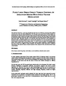
Methodology The top level view of the electric vehicle model used in this paper is shown in Fig. 1. The FL speed controller generates accelerator pedal or brake pedal angles α and β respectively to control the vehicle’s speed. The current control ∗ ∗ compares the target supply currents 𝑖𝑑𝑠 and 𝑖𝑞𝑠 with the measured stator currents to produce supply voltages 𝑣𝑑𝑠 and 𝑣𝑞𝑠 . The same top level model can be used for both IM and PMSM models by adjusting the mathematical equations where required.
Both IM and PMSM models use vector control to simplify the 3 phase AC circuits into a 2 phase dq-axis model, where the d-axis usually regulates the motor flux and the q axis determines the torque output.
Fig. 1 - Top Level Vehicle Model The IM is represented by the differential equations (1)-(4) which calculates the dq-axis flux linkages 𝜆𝑑𝑠 , 𝜆𝑞𝑠 , 𝜆𝑑𝑟 , and 𝜆𝑞𝑟 using the motor winding resistance 𝑟𝑠 , rotor resistance 𝑟𝑟 , number of magnetic poles 𝑃, electrical angular velocity 𝜔𝑒 , and rotor angular velocity 𝜔𝑟 (Pahwa, 2009; Leedy, 2013). 𝑑𝜆𝑑𝑠 − 𝜔𝑒 𝜆𝑞𝑠 𝑑𝑡 𝑑𝜆𝑞𝑠 𝑣𝑞𝑠 = 𝑟𝑠 𝑖𝑞𝑠 + + 𝜔𝑒 𝜆𝑑𝑠 𝑑𝑡 𝑑𝜆𝑑𝑟 = 0 = 𝑟𝑟 𝑖𝑑𝑟 + − (𝜔𝑒 − 𝜔𝑟 )𝜆𝑞𝑟 𝑑𝑡 𝑑𝜆𝑞𝑟 = 0 = 𝑟𝑟 𝑖𝑞𝑟 + + (𝜔𝑒 − 𝜔𝑟 )𝜆𝑑𝑟 𝑑𝑡
(1)
𝑣𝑑𝑠 = 𝑟𝑠 𝑖𝑑𝑠 +
𝑣𝑑𝑟 𝑣𝑞𝑟
(2) (3) (4)
The inductance linkage equations (5)-(6) require the leakage inductance of the stator 𝐿𝑙𝑠 , rotor 𝐿𝑙𝑟 , and the magnetising inductance 𝐿𝑚 of the motor to be used in equations (7)-(10) to find the dq-axis currents 𝑖𝑑𝑠 , 𝑖𝑞𝑠 , 𝑖𝑑𝑟 and 𝑖𝑞𝑟 . The IM torque output 𝑇𝑒 is then calculated using equation (11).
𝑇𝑒 =
𝐿𝑠 = 𝐿𝑚 + 𝐿𝑙𝑠
(5)
𝐿𝑟 = 𝐿𝑚 + 𝐿𝑙𝑟
(6)
𝑖𝑑𝑠 =
𝜆𝑑𝑠 − 𝐿𝑚 𝑖𝑑𝑟 𝐿𝑠
(7)
𝑖𝑞𝑠 =
𝜆𝑞𝑠 − 𝐿𝑚 𝑖𝑞𝑟 𝐿𝑠
(8)
𝑖𝑑𝑟 =
𝜆𝑑𝑟 − 𝐿𝑚 𝑖𝑑𝑠 𝐿𝑟
(9)
𝑖𝑞𝑟 =
𝜆𝑞𝑟 − 𝐿𝑚 𝑖𝑞𝑠 𝐿𝑟
(10)
3𝑃 𝐿 (𝑖 𝑖 − 𝑖𝑑𝑠 𝑖𝑞𝑟 ) 4 𝑚 𝑞𝑠 𝑑𝑟
(11)
An estimate of the electrical angular speed 𝜔𝑒 can be found from equations (12)-(14) utilising feedback from the vehicle model to find the traction motor’s mechanical speed 𝜔𝑚 and electrical rotor speed 𝜔𝑟 (Deshpande, 2013). Equation (12) can be re-arranged to produce the estimated rotor flux value 𝜑𝑟 , which will also be fed-back to the FL flux controller. 𝐿𝑟 𝑑𝜑𝑟 + 𝜑𝑟 = 𝐿𝑚 𝑖𝑑𝑠 𝑅𝑟 𝑑𝑡 𝑃𝜔𝑚 𝜔𝑟 = 2 𝐿𝑚 𝑅𝑟 𝑖𝑞𝑠 ) ( ) + 𝜔𝑟 𝜔𝑒 = ( 𝐿𝑟 𝜑𝑟
(12) (13) (14)
Up to base speed 𝜔𝑏 , the IM will have a constant target rotor flux 𝜑 ∗ given by equation (15)-(16), leaving the q-axis current to be limited by the rated stator current 𝑖s in equation (17). Above base speed, the target flux reduces proportionally with speed. Equation (14) is dependent on the rated supply frequency 𝑓, nominal no-load voltage 𝑉𝑛𝑓 , and a scaling factor 𝑘 (Kim, 1997; Mengoni, 2007; Xie, 2015). 𝑉𝑛𝑓 2𝜋𝑓𝐿𝑚 𝑖𝑑∗ = {
𝜔𝑚 ≤ 𝜔𝑏
𝑉𝑛𝑓 𝜔𝑏 𝑘 [ ] 2𝜋𝑓𝐿𝑚 𝜔𝑚
(15) 𝜔𝑚 > 𝜔𝑏
𝜑 ∗ = 𝐿𝑚 𝑖𝑑∗
(16)
∗ 2 ∗ 𝑖𝑞𝑠 = √𝑖s2 − 𝑖ds
(17)
The PMSM can be represented by the differential equations (18)-(21) using permanent magnet flux 𝜑𝑚 , since there is no rotor slip, 𝜔𝑒 = 𝜔𝑟 (Morimoto, 1990; Mahammadsoaib, 2015). The IPMSM torque output is given by equation (22). 𝑑𝜆𝑞𝑠 + 𝜔𝑒 𝜆𝑑𝑠 𝑑𝑡 𝑑𝜆𝑑𝑠 = 𝑟𝑆 𝑖𝑑𝑠 + − 𝜔𝑒 𝜆𝑞𝑠 𝑑𝑡
𝑣𝑞𝑠 = 𝑟𝑆 𝑖𝑞𝑠 +
(18)
𝑣𝑑𝑠
(19)
𝑇𝑒 =
𝜆𝑞𝑠 = 𝐿𝑞 𝑖𝑞
(20)
𝜆𝑑𝑠 = 𝐿𝑑 𝑖𝑑 + 𝜑𝑚
(21)
3𝑃 (𝑖 𝜑 − 𝑖𝑞𝑠 𝑖𝑑𝑠 (𝐿𝑞 − 𝐿𝑑 )) 4 𝑞𝑠 𝑚
(22)
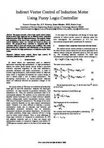
∗ Maximum Torque Per-Amp (MTPA) control utilises the motor’s saliency 𝜀 to use 𝑖𝑑𝑠 to contribute ∗ output reluctance torque, in addition to flux linkage control. Under MTPA control, 𝑖𝑑𝑠 becomes dependent on the torque demand 𝑖𝑞∗ from the FL speed controller and the rotor speed, as shown by (Morimoto, 1990; Miraeian, 2011; Jung, 2015). Equation (23) finds a suitable limit 𝑖𝑞∗ 𝑚𝑎𝑥 for each rotor speed at full load using rated current 𝑖𝑠 . Fig. 2 outlines the process involved to regulate 𝑖𝑑∗ from equations (24)-(25). This process accounts for the MTPA control region below base speed, the partial-flux weakening, and full-flux weakening region above base speed. The partial flux weakening region lies between 𝜔𝑏 and the critical speed 𝜔𝑐 set by equation (26).
𝜑 − √𝜑2 + 8(𝐿𝑞 − 𝐿𝑑 )2 𝑖𝑠2 4(𝐿𝑞 − 𝐿𝑑 ) ∗ 𝑖𝑞𝑠 𝑚𝑎𝑥 =
𝜔𝑚 ≤ 𝜔𝑏
𝜑 1 𝜀𝜑 2 𝑉 2 2 − 1) ((𝜀𝑖 )2 − ( 𝑛 ) )] 𝜔 ≥ 𝜔 − √( (𝜀 [ ) + 𝑠 𝑚 𝑏 𝜀 2 − 1 𝐿𝑑 𝐿𝑑 𝜔𝑒 𝐿𝑑
(23)
{
∗ 𝑖𝑑𝑠 =
𝜑 𝜑2 2 −√ + 𝑖𝑞𝑠 2(𝐿𝑞 − 𝐿𝑑 ) 4(𝐿𝑞 − 𝐿𝑑 )2
∗ 𝑖𝑑𝑠 =−
(24)
𝜑 1 𝑉2 + √ 2 − (𝐿𝑞 𝑖𝑞 )2 𝐿𝑑 𝐿𝑑 𝜔𝑒 𝜔𝑐 =
(25)
𝑉 𝑃𝜑
(26)
Fig. 2 - IPMSM id* Flow chart The FL current controllers output d-q axis stator voltages 𝑣𝑑𝑠 and 𝑣𝑞𝑠 respectively for their individual control circuits. Decoupling voltages in equation (27)-(28) are added to the output from the FL current controller (Morimoto, 1994). As the magnitude between 𝑣𝑑𝑠 and 𝑣𝑞𝑠 approaches the maximum supply voltage 𝑉, 𝑣𝑑𝑠 is given priority and 𝑣𝑞𝑠 becomes limited. −𝜔𝑒 𝐿𝑠 𝑖𝑞𝑠 (1 − 𝑣𝑑𝑠 = {
−𝜔𝑒 𝐿𝑞 𝑖𝑞𝑠
𝜔𝑒 𝐿𝑠 𝑖𝑑𝑠 (1 − 𝑣𝑞𝑠 =
𝐿2𝑚 ) 𝐿𝑠 𝐿𝑟
𝐼𝑀 (27) 𝑃𝑀𝑆𝑀
𝐿2𝑚 𝐿𝑚 ) + 𝜔𝑒 𝜆 𝐿𝑠 𝐿𝑟 𝐿𝑟 𝑑𝑟
{ 𝜔𝑒 𝐿𝑑 𝑖𝑑𝑠 + 𝜔𝑒 𝜑𝑚
𝐼𝑀
𝑃𝑀𝑆𝑀
(28)
All the FL controllers in this paper use the same input and output membership function shapes shown in Fig. 3, however with different input/output ranges suitable to the specific application.
Fig. 3 - FL input membership functions The FL speed controller has 2 inputs; velocity error and change in velocity error with the corresponding rule bases in Table I. This FLC provides appropriate accelerator or brake pedal angles comparable to a real driver’s response, thus producing close representations of how the vehicle behaves in real world scenarios. Input 1 has an input range of ±1 kph and input 2 has an input range of ±10 kph·s-1. The FL speed controller outputs values in the range of ±100 % pedal movement, where positive values represent the accelerator pedal movement and negative values are for the brake pedal. Table I - Speed FL Rule Base 𝐄𝐫𝐫𝐨𝐫
𝐎𝐮𝐭𝐩𝐮𝐭
𝐝(𝐄𝐫𝐫𝐨𝐫) 𝐝𝐭
-3
-2
-1
0
1
2
3
-3
-1
0
0
1
2
3
3
-2
-1
-1
0
0
1
2
3
-1
-2
-2
-1
0
1
2
3
0
-2
-2
-1
0
1
2
3
1
-3
-2
-1
0
1
2
2
2
-3
-2
-1
0
0
1
2
3
-3
-3
-2
-1
00 1
Similar to the FL speed controller, the induction motor incorporates a FL flux controller to maintain the motor flux. The FL flux controller also has 2 inputs; flux error with an input range of ±0.05 Wb, and change in flux error with an input range of ±10 Wb·s-1. The rule base for the FL flux controller is shown in Table II. The controller output is in the range ±𝑖𝑠 A, allowing for a large current can be supplied when the error is large to quickly increase the flux value.
Table II - Flux FLC Rule Base 𝐄𝐫𝐫𝐨𝐫
𝐎𝐮𝐭𝐩𝐮𝐭
𝐝(𝐄𝐫𝐫𝐨𝐫) 𝐝𝐭
-3
-2
-1
0
1
2
3
-3
-1
0
1
2
3
3
3
-2
-2
-1
0
1
2
3
3
-1
-2
-2
-1
0
1
2
3
0
-3
-2
-1
0
1
2
3
1
-3
-2
-1
0
1
2
2
2
-3
-3
-2
-1
0
1
2
3
-3
-3
-3
-2
-1
0
1
For simplicity, the FL current controller use the instantaneous current error as its only input in the range ±1 A. The FL current controller’s output is in the range of ±𝑉𝑚𝑎𝑥 V allowing the current to rise quickly when the error is large. The rules base for the FL current controller is shown in Table III. Table III - Current FLC Rule Base 𝐄𝐫𝐫𝐨𝐫 𝐎𝐮𝐭𝐩𝐮𝐭
-3
-2
-1
0
1
2
3
3
2
1
0
-1
-2
-3
A vehicle model combining the net forces acting on the vehicle including the traction force 𝐹𝑇𝑟𝑎𝑐𝑡𝑖𝑜𝑛 , brake force 𝐹𝐵𝑟𝑎𝑘𝑒 , rolling resistance 𝐹𝑅𝑜𝑙𝑙𝑖𝑛𝑔 , and aerodynamic drag 𝐹𝐴𝑒𝑟𝑜 from equations (29)-(31) predicts the vehicle’s longitudinal dynamics. 𝐹𝑇𝑟𝑎𝑐𝑡𝑖𝑜𝑛 is calculated from the motor torque 𝑇𝑒 , final drive ratio 𝑁𝑓𝑑 , final drive efficiency 𝜂𝑓𝑑 and wheel radius 𝑟𝑤 (Gillespie, 1992; Osorio, 2012). 𝐹𝑅𝑜𝑙𝑙𝑖𝑛𝑔 is reliant on the coefficients of rolling resistance 𝑓𝑟 , the mass the vehicle 𝑀 and gravity 𝑔. 𝐹𝐴𝑒𝑟𝑜 is dependent on the frontal area of the vehicle 𝐴, coefficient of drag 𝐶𝐷 , density of air 𝜌 and the speed of the vehicle 𝑈. 𝐹𝑇𝑟𝑎𝑐𝑡𝑖𝑜𝑛 =
𝑇𝑒 𝑁𝑓𝑑 𝜂𝑓𝑑 𝑟𝑤
(29)
𝐹𝑅𝑜𝑙𝑙𝑖𝑛𝑔 = 𝑓𝑟 𝑀𝑔
(30)
1 𝐹𝐴𝑒𝑟𝑜 = 𝐶𝐷 𝜌𝐴𝑈2 2
(31)
Using the brake pedal angle from the FL speed controller, the brake force 𝐹𝐵𝑟𝑎𝑘𝑒 can be found from a brake pedal angle – brake force lookup table. The behaviour of the brake pedal is linear from no brake force at 0% brake pedal angle, and FBmax at 100%. The effective mass of the vehicle 𝑀𝑟 due to the rotational inertia of the rotor 𝐼𝑚 , final drive 𝐼𝐹𝑑 and wheel 𝐼𝑊ℎ is found in equation (32). 2 2 𝑀𝑟 = (𝐼𝑚 𝑁𝑓𝑑 + 𝐼𝐹𝑑 𝑁𝑓𝑑 + 𝐼𝑊ℎ )
1 𝑟𝑤 2
(32)
Equation (33) combines the forces acting on the vehicle and the effective vehicle mass to calculate the acceleration of the vehicle 𝑎𝑥 and thus the vehicle’s velocity. The mechanical rotational speed of the rotor can be found using equation (34). 𝐹𝑇𝑟𝑎𝑐𝑡𝑖𝑜𝑛 − 𝐹𝐵𝑟𝑎𝑘𝑒 − 𝐹𝐴𝑒𝑟𝑜 − 𝐹𝑅𝑜𝑙𝑙𝑖𝑛𝑔 = (𝑀 + 𝑀𝑟 )𝑎𝑥 𝜔𝑚 =
𝑈𝑁𝑓𝑑 𝑟𝑤
(33) (34)
III.
Results To show the flexibility of the FL control scheme, the same FL speed and FL current controllers were used to control a vehicle using a single IPMSM and an identical vehicle using a dual hub IM with an additional flux controller. The motor parameters are listed in Table IV and the vehicle parameters in Table V. The model can be adapted for dual hub motors by doubling the IM motor torque output. Table IV - Motor Parameters Parameter Nominal rated power (kW) Rated Voltage (V) Rated Current (A) Base Speed (rpm) Maximum speed (rpm) Stator resistance (mΩ) Rotor resistance (Ω) Number of Poles D-axis inductance (mH) Q-axis inductance (mH) Rotor magnetic flux (Wb) Stator leakage inductance (mH) Rotor leakage inductance (mH) Magnetizing inductance (mH) Rotor Inertia (kg·m-2)
IPMSM 100 155 450 3000 6500 8.296 8 1.742 2.927 0.071 0.5
IM 38 460 55 1700 5350 87 228 4 0.8 0.8 34.7
Table V - Vehicle parameters Parameter Vehicle Mass (kg) Coefficient of Drag Frontal Area (m2) Wheelbase (m) Wheel Radius (m) Coefficient of rolling resistance (%) Wheel Inertia (kg·m2) Brake pedal max force (N) Final drive efficiency Final drive inertia (kg·m2) Air density (kg·m-3)
Value 1600 0.27 2.5 2.6 0.32 2 0.8 800 0.98 0.1 1.22
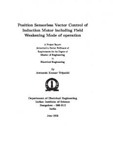
The vehicle simulations followed a section of the New European Drive Cycle (NEDC) to show how the motors and control systems perform. Fig. 4a and Fig. 5a show the vehicle’s speed profiles using the dual hub IM and single IPMSM respectively using both PI and FL speed control. The FLC showed improved dynamic performance over the PI speed controller by controlling the vehicle like a real driver would. The FLC did not overshoot the target speed, it was able to anticipate changes in the target speed ahead of time and had a faster reaction to target speed step changes. This behavior was experienced with both IM and IPMSM vehicles because as with a person driving the vehicle the control principles remain the same. The accelerator and brake pedal response for the FLC showed that as the vehicle approached the target speed, the accelerator pedal would slowly reduce in angle until it reaches its steady-state value, whereas the PI controller would overshoot the target speed and have to apply the brake pedal. Fig. 4b and Fig. 4c show the d-q axis current control for the FLC and PI respectively for the dual hub IM vehicle, Fig. 5b and Fig. 5c show similar results for the IPMSM vehicle. The PI and FL current control methods showed satisfactory results meeting the target current with minimal error and acceptable voltage outputs. Fig. 4d shows the PI and FL flux control used in the IM. The simulations showed that the flux reached its target value sooner, than if a constant d-axis current was used on start-up. However, the PI controller overshot the target flux, which may push the motor’s flux into saturation, creating greater inefficiencies.
a)
b)
c)
d) Fig. 4 - Dual hub IM vehicle a) Speed Control comparison, b) FL Current control c) PID Current Control d) Flux control comparison
a)
b)
c) Fig. 5 - Single IPMSM vehicle a) Speed Control comparison, b) FL Current control c) PID Current Control IV.
Conclusion In this paper, a fuzzy logic based control scheme has been presented that is capable of the speed, current, and flux control of any electric vehicle using an IM or IPMSM. The fuzzy controllers showed superior performance over their PID counterparts with a reduction in overshoots, fast response times and a better representation of how the vehicle would perform in real world scenarios. Furthermore the fuzzy logic scheme did not require re-tuning between experiments, highlighting the convenience of this control scheme to vehicle designers as it will save time otherwise spent re-tuning PID controllers. V. References Adhavan, B., 2011. Field Orientated Control of Permanent Magnet Synchronous Motor (PMSM) using fuzzy logic controller. Trivandrum, Recent Advances in Intelligent Computational Systems. Anon., 2011. Benefits of cleaner vehicles. [Online] Available at: https://climate.nasa.gov/news/502/benefits-of-cleaner-vehicles/ [Accessed 14 03 2017]. Bolognani, S., 2011. Flux-weakening in IPM motor drives: Comparison of state-of-art algorithms and a novel proposal for controller design. Birmingham, European Conference on Power Electronics and Applications . Bose, B. K., 2002. Modern Power Electronics and AC Drives. Knoxville: Pretice-Hall. Casadei, D., 2008. Field-weakening control schemes for high-speed drives based on induction motors: a comparison. Power Electronics Specialists Conference 2008, pp. 2159-2166. Deshpande, G., 2013. Speed Control of Induction Motors using Hybrid PI plus Fuzzy Controller. International Journal of Advances in Engineering and Technology, 6(5), pp. 2253-2261. Emadi, A., 2005. Topological overview of hybrid electric and fuel cell vehicular power system architectures and configurations. IEEE Transactions on Vehicular Technology, 54(3), pp. 763 - 770. Evangeloou, S., 2016. Dynamic modeling platform for series hybrid electric vehicles. Florianopolis, Internaional Federation of Automatic Control. Fahassa, C., 2015. Improvement of the Induction Motor Drive Indirect Field Orientated Control Performance by Substuting its Speed and Current Controllers with Fuzzy Logic Components. Marrakech, 2015 3rd International Renewable and Sustainable Energy Conference. Gillespie, T. D., 1992. Fundamentals of Vehicle Dynamics. Warrendale: Inc Society of Automive Engineers. Jalaifar, M., 2006. Dynamic Modelling and simulaiton of an Induction Motor with Adaptive Backstepping Design of an Input-Output Feedback Linearization Controller in Series Hybrid Electric Vehicle. Delhi, s.n. Jung, S.-Y., 2015. Torque Control of IPMSM in the Field Weakening Region with Improved DC-Link Voltage Utilization. IEEE Transactions on Industrial Electronics , 62(6), pp. 3380 - 3387. Kim, J.-M., 1997. Speed Control of Interior Permanent Magnet Synchronous Motor Drive for the Flux Weakening Operation. IEEE Transactions on Industry Applications, 33(1), pp. 43 - 48. Kodaoda, K., 2002. Fuzzy Speed and Steering Control of an AGV. IEEE Transactions on Control Systems Technology, 10(1), pp. 112-120. Leedy, A., 2013. Simulink/MATLAB Dynamic Induction Motor Model for Use as A Teaching and Research Tool. International Journal of Soft Computing and Engineering, 3(4), pp. 2231-2307.
Mahammadsoaib, S., 2015. Vector controlled PMSM drive using SVPWM technique - A MATLAB / simulink implementation. Visakhapatnam, s.n. Mengoni, M., 2007. Stator Flux Vector Control of Induction Motor Drives in the Field-Weakening Region. Miraeian, B., 2011. A comparative study of various intelligent based controllers for speed control of IPMSM drives in the field weakening region. Expert Systems with Applications, 38(10), p. 12643–12653. Morimoto, S., 1990. Expansion of operating limits for permanent magnet motor by current vector control considering inverter capacity. IEEE Transactions on Industry Applications, 26(5), pp. 866-871. Morimoto, S., 1994. Effects and Compensation of Magnetic Saturation in Flux-Weakening Controlled Permanent Magnet Synchronous Motor Drives. IEEE Transactions on Industry Applications, pp. 1632-1637. Osorio, J., 2012. Electric Vehicle Powertrain Control with Fuzzy Indirect Vector Control. San Luis Potosí, Advances in Artificial Intelligence and Applications, pp. 122-127. Pahwa, V., 2009. Transient anslysis of three-phase induction machine using different reference frames. Journal of Engineering and Applied Sciences, 4(8), pp. 31-38. Uddin, M., 2002. Performance of Fuzzy-Logic-Based Indirect Vector Control for Induction Motor Drive. IEEE Transactions on Industry Applications, 38(5), pp. 1219-1225. Xie, P., 2015. Research on field-weakening control of induction motor based on torque current component of the voltage closed-loop. Auckland, s.n., pp. 1618-1621. Yilmaz, M., 2015. Limitations/capabilities of electric machine technologies and modelling approaches for electric motor design analysis in plug-in electric vehicle applications. Renewable and Sustainable Energy Reviews, 52(1), pp. 88-99. Zhou, Q., 2017. Intelligent sizing of a series hybrid electric power-train system based on Chaos-enhanced accelerated particle swarm optimization. Applied Energy, 189(1), pp. 588-601.