TEX10. 1. TEX9. 1. TEX11. Cells Texture ! ! Cells Texture. (a). (b). Fig. 5. Two different approaches to parallelize random number generations in GPU. (a) Each ...
Generating Massive High-Quality Random Numbers using GPU Wai-Man Pang
Tien-Tsin Wong
Abstract— Pseudo-random number generators (PRNG) have been intensively used in many stochastic algorithms in artificial intelligence, computer graphics and other scientific computing. However, the current commodity GPU design does not facilitate the efficient implementation of high-quality PRNGs that require high-precision integer arithmetics and bitwise operations. In this paper, we propose a framework to generate a high-quality PRNG shader for all kinds of GPUs. We adopt the cellular automata (CA) PRNG to facilitate high speed and parallel random number generation. The configuration of the CA PRNG is completed automatically by optimizing an objective function that accounts for quality of generated random sequences. To visually evaluate the result, we apply the best PRNG shader to photon mapping. Timing statistics show that our GPU parallelized PRNG is much faster than a pure CPU implementation.
Pheng-Ann Heng
systems or games. They usually cannot afford a heavy loading PRNG. Therefore, we propose a fast GPU-based PRNG which generates thousands of pseudo random numbers in parallel. Our PRNG is based on cellular automata (CA). CA-based PRNG does not require high-precision integer arithmetics nor bitwise operations. It relies only on simple low-precision arithmetic and interconnection of cells (pixels). Therefore, it fits nicely to the architecture of the GPU. The quality of PRNG is ensured by optimizing the CA-based PRNG model, so that random sequences have long repeating cycle and low correlations among themselves. Experiments show that our GPU-based CA-PRNG is significantly faster than a pure CPU-based one.
I. I NTRODUCTION NIFORMLY distributed random numbers are essential in many evolutionary computing algorithms. It is important that they are high quality and can be generated quickly. Moreover, a huge amount of random numbers is usually required in the process. Therefore, a natural and practical solution to generate these random numbers is using the programmable graphics processing unit (GPU), which is commonly equipped on ordinary PCs nowadays. GPU is a SIMD-based parallel processor tailormade for graphics programming. Unfortunately, current GPUs are not provided with any high-quality pseudo-random number generator (PRNG). A direct porting of most conventional PRNG to GPU is not feasible, because most current GPUs does not support high-precision integer arithmetics and native bitwise operations. For example, the rand() in standard C library is an implementation of linear congruential generator (LCG) which requires high-precision integer arithmetics like 32 or 64-bit modulo. The quality of random numbers produced is an essential property for any PRNG, it can directly affect the result or convergence rate of certain stochastic algorithms. However, it is difficult to evaluate the quality of random sequences produced by PRNGs analytically. Moreover, the way of using random sequence can significantly affect the randomness provided by a PRNG, including actual used bits of random numbers and PRNG on parallel computers [1]. Therefore, people rely on testing the length of repeating cycle and the correlation between sub-sequences under many utilization scenarios, in order to empirically examine the qualities. Speed is another important concern when designing PRNG, especially for real-time applications like scientific
U
The authors are with Department of Computer Science and Engineering, The Chinese University of Hong Kong, Shatin, New Territories, Hong Kong (email: {wmpang, ttwong, pheng}@cse.cuhk.edu.hk)
II. R ELATED W ORK The generation of uniformly distributed random number sequence has been actively studied in the last decade. Algorithms like linear congruential generator, lagged Fibonacci generator, linear feedback shift register generator [2] usually require very simple arithmetics such as addition, modulo or bitwise operations. However, many of these early PRNG have deficiencies [3], [4], [5]. Modern PRNG like the Mersenne Twister [6] does not suffer from these deficiencies, but it is more complex and depends heavily on bitwise operations. CA-based PRNG is proposed by Wolfram [7]. The first suggested CA-based PRNG is a 1D cellular automata with a neighborhood size of three. Because of the simple structure but amazing randomness it produces, CA-based PRNG is being studied thoroughly, especially in the area of hardware implementation of PRNG. Other efficient models of CAbased PRNG have been proposed [8], [9]. Because of its strong randomness and not requiring high-precision integer arithmetics nor bitwise operations, we choose CA-based PRNG for the GPU implementation. Many large-scale Monte Carlo simulations run on parallel computers, generating random numbers in parallel manner is another widely discussed topic [10], [11]. Common methods include cycle division and sequence splitting to divide the original serial sequence into separated ones and run on different processors [1]. Two quality requirements are especially important for parallel PRNG, these include the intra-stream and inter-stream correlations. The intra-stream correlation refers to the correlation within a random sequence produced from the same processor. While the inter-stream correlations are between sequences from different processors. Many of the traditional PRNGs fail to work well under a parallel environment, especially suffer from the inter-stream correlation [11].
841 c 978-1-4244-1823-7/08/$25.00�2008 IEEE
III. CA- BASED PRNG A. Basics CA-based PRNG was first proposed by Wolfram [7]. The basic structure of CA-based PRNG is analogous to a generic cellular automata. An example is illustrated in Figure 1. It consists of an array of interconnected cells, each with homogeneous behavior. Each cell holds a cell state which corresponding to a particular bit in the generated random number. Therefore, the number of cells have to be adjusted depending on the possible outcomes of random numbers. Usually, the number of cells used will be larger than the number of bits required for the random number. Only selected bits are outputted, this brings better randomness [7]. The connectivity among interconnected cells is defined local to the cell. We consider a simple CA of only 4 cells, namely A, B, C, and D in Figure 1. Each cell connects to its left cell and the second right cell, in this case the connectivity is denoted as (-1,2). Notice that the connectivity wraps around when connected to an out-of-boundary cell. For example, left connection of cell A goes to cell D and cell D’s second right connection should be cell B. A cell equation Φ is defined for all cells in a CA-based PRNG. Each time the next random number is generated, each cell updates its own state by computing this cell equation Φ at the same time. As illustrated in Figure 2, the cell equation Φ takes cell state values ci from its connected neighbors as input parameters, and output a single bit as the cell state. The cell equation can be represented mathematically as Equation 1. cgi represents the i-th cell state at the gth iteration and nj means the offset to the j-th connected neighbors. Notice that the neighborhood of a cell can include the cell itself. In addition, the input neighboring cell state values ci all come from previous cell state (g − 1) only, so there is no ambiguity during simultaneous update of cell states. After all cells update their states, a new random number is obtained by collecting the bits scattered among the cells. g−1 g−1 (1) cgi = Φ(cg−1 i+n0 , ci+n1 , ..., ci+nj ) We demonstrate with a 4-cell PRNG in Figure 3 to clarify the mechanism of random number generation from CA-based PRNG. This 4-cell PRNG outputs a 3-bit random number by gathering the state values from cells A, C and D. The cell connectivity and cell equation is defined as (-1,2) and Φ = step(1, 3 − c−1 − 2c2 ). Function step(a, x) returns 1 if x ≥ a , otherwise 0. Similar to all other PRNGs requiring an initial seed, CA-based PRNG also requires an initialization of cell states. We can simply initialize them with arbitrary bits as in Figure 3(a). In the process of producing the next random number, all cell states are updated simultaneously. The first computed result and the corresponding new random number is shown in Figure 3(b). Therefore, cell A has cells C and D as its neighbors. By passing the previous state values of cell C and D, that is 0 and 1 respectively (Figure 3(a)), to the cell equation Φ; it updates the state of cell A to 1, as shown in Figure 3(b). Other cells work similarly and simultaneously.
842
Fig. 1. A four-cell CA-based PRNG with connectivity of (-1,2). Connections are wrap-around.
When all cell states are updated using the cell equation, a new random number can be obtained by collecting the cell states of A, C and D, with state of cell A as the MSB and state of cell D as the LSB. Hence we get a random number of 111 = 7 (Figure 3(b)). Repeating the same process will generate the next random number. Figure 3(c) shows one more iteration and the corresponding random number is 011 = 3. The structural design of CA-based PRNG is rather simple and very suitable to be implemented on GPU. Especially, all cells are working homogeneously and independently fits nice to the GPU architecture. In the following section, we are going to discuss issues concerning the GPU implementation in more details.
Fig. 2.
An example cell of CA-based PRNG.
Fig. 3. Three iterations of generating 3-bit random number with the 4-cell CA-based PRNG.
B. Shader Implementation The GPU implementation of CA-based PRNG as a shader is straight-forward. Each cell resembles to a texel in the texture, while the cell equation Φ is computed inside the shader code. The connectivity of neighboring cells is done based on texture reference. Since cells are independent of each other, it works in a similar manner as the fragment shader in GPUs. The pseudo fragment shader code in Algorithm 1 demonstrated an implementation of the CA-based
2008 IEEE Congress on Evolutionary Computation (CEC 2008)
PRNG. Sample Cg shader programs of CA-based PRNG can be found in the appendix.
Texture coordinate :
cells:
(0,0) (1,0) (2,0) (3,0)
0
1
0
(62,0) (63,0)
0
1
MSB Cell 0 Cell 1 Cell 2 Cell 3
In Algorithm 1, the cells is the 2D texture storing all the cell states in previous iteration. It is initialized with arbitrary values assigned by user or randomly before executing the shader. The neighbors here represents the connectivity configuration, for example, it is (-1,2) in the CA-based PRNG demonstrated in Figure 3. First, the shader fetches the neighbor cell states by offsetting the current texture coordinate according to the connectivity configuration (neighbors). By offsetting current texture coordinate (texcoord) by n, we have the correct texture coordinate of the neighbor cell states. Since the connectivity is wrap-around when out of boundary, we need to modular it by number of cellularautomata (CA SIZE). Then, all the neighbor cell states are put in the array nbrCellstates. Passing all collected previous cell states from the neighbors (nbrCellstates) to the cell equation (celleqn), the returned value is the new state of current cell (newCellState). This is stored to the output texture and the roles of newCellState and cells are then interchanged in the next iteration. The computation of cell equation can be performed in fragment shader. In fact, we speed up the evaluation of cell equation by replacing complicated cell equation with a lookup table. Since the cell equation is actually a mapping of neighbor cell states to an output state which is either 1 or 0, we can precompute the cell equation and store it in a lookup table (texture) to achieve a speed-up. A straightforward implementation is to use a ndimensional texture if there are n neighbor connections. However, high-dimensional table is currently not supported on GPU if the table dimension exceeds 3. Alternatively, we can pack the n bits to form a n-bit index and the precomputed values are stored in a 1D texture only. In a 4-connected CAbased PRNG, we need only 24 = 16 different output states, so a 16-entry lookup table is sufficient. Figure 4 shows the organization of cell states (cell) and lookup tables (eqnLUT) in texture. Figures 4(a) and 4(b) show the data organization of the 64 cell states in textures (cells) and the 16-entry lookup table (eqnLUT) respectively. The state of cells are tightly packed and stored in a texture. The random number is formed by packing the 32 cell states as in Figure 4(c). As the bits of random number being generated are scattered among different cells (texels), we have to reorganize them to form the 32-bit integer number. However, GPU does
LSB
(a)
Algorithm 1 Pseudo code of CA-based PRNG Shader % Collect all the neighboring cell states Foreach n in neigbhors nbrT excoord ← (texcoord − n) mod CA SIZE nbrCellstates[n] ← texRECT (cells, nbrT excoord) End Foreach % Call the cell equation here newCellState ← celleqn(nbrCellstates);
1
Cell 62 Cell 63
Texture coordinate :
(0,0) (1,0) (2,0)
eqnLUT: 1
0
(15,0)
0
1
Cell equation input parameters : (0,0,0,0) (0,0,0,1) (0,0,1,0)
(1,1,1,1)
(b) Texture coordinate :
(1,0) (3,0) (5,0)
(61,0) (63,0)
Random number : 1 0 0 formation MSB Cell 1 Cell 3 Cell 5
1
1
Cell 61 Cell 63
LSB
(c)
Fig. 4. Data organization in the textures for a 4 connected 64 cells CAbased PRNG. (a) Cell organization and (b) lookup table for evaluating the cell equation. (c) Formation of random number by 32 cell states.
not support high-precision integer values, we need to use floating point to hold the high-precision integer for output. One way to do so is to convert the generated random number bits, ri , to a floating point value, f , as Equation 2. The corresponding shader (pack) can refer to appendix. (2) f = (((r0 /2) + r1 )/2 + ... + r31 )/2 Another way to store the random numbers is directly storing all the bits inside the floating point values by using the mantissa part only. Since each floating point has 23-bit for mantissa, each pixel can store two 32-bit random numbers instead of 4. Then, each 32-bit integer random number is repacked in CPU. IV. Q UALITY O PTIMIZATION The particular connectivity and cell equation demonstrated in Figure 3 is only one of the many possible configurations. There are many possible configurations of a CA-based PRNG and they affect the quality of random numbers generated. The variable factors include connectivity, cell equation and even the number of cells used. However, it is difficult to find the best configuration analytically. The number of possible configurations increases exponentially with the number of cell and number of connectivities used. Therefore, searching a good configuration by brute-force searching is not effective. We can employ an optimization method based on heuristic to improve the searching speed. In order to make the optimization problem tractable. We fixed the size of CA to be 64 and the number of neighborhood to 4. Only even-numbered cells are extracted to form a random number. The neighborhood connection and cell equation Φ is left to the optimization. We find that this restriction does not affect much the quality of PRNG but it substantially reduces the search space. We encode each CA-based PRNG candidate by its connectivities and cell equation. As the cell equation can be represented with a lookup table in 2n bits, where n is the connectivities; therefore, 2n + n bits are sufficient to encode a candidate. Then, the optimization is carried out using genetic algorithm. The objective function is defined to evaluate the
2008 IEEE Congress on Evolutionary Computation (CEC 2008)
843
quality of generated random sequence. The optimization starts from an initial population of candidates with different configurations. In each generation, candidate with the highest score is chosen as the best candidate. Next, a new population is generated using crossover and mutation operators. Crossover tries to combine features from 2 selected parents to reproduce a new one. The crossover point is randomly chosen within the cell equation Φ. Mutation picks a selected candidate and randomly alters the cell equation. The selection of parent candidates is based on tournament scheme. It first chooses a subset of candidates randomly, then the best candidate within the subset is selected for crossover. The new population is again evaluated using the objective function, the process repeats until certain number of generations is reached or the result converges. A. Objective Function The definition of objective function is the most essential part in our optimization framework, because it directly affects the final results. The objective function is : (3) objective = w0 × e + w1 × ϕ where e is the entropy, ϕ is the overall p-value from random number quality test. w0 and w1 are weights (w0 = 0.5, w1 = 0.5). Higher weights should be given to w1 for scientific applications. Entropy e is the normalized k-bit entropy computed from sub-sequences of random numbers [12], �2k −1 − i=0 pi log pi e= (4) k where pi is the occurrence of the binary value of subsequence i. In our experiments, 16-bit entropy is used. Therefore, we get i by extracting 32 different 16-bits subsequences from the 32-bits generated random number (bits are wrap-around when out-of-boundary). Besides entropies, there is an even more robust empirical test designed for measuring the quality of random sequences. It is called the DIEHARD test [13]. ϕ is the overall p-value from DIEHARD. It is a set of stringent tests [2] which is a more strict test specific for random number sequences. The DIEHARD suite has totally 14 tests, namely birthday spacing test, GDC Test, gorilla test, overlapping permutation test, rank of matrix test, monkey test, count the 1’s test, parking lot test, minimum distance test, random sphere test, squeeze test, overlapping sums test, runs up and down test and the craps test. The basic idea of these tests are similar. First, they try to extract various subsets of bits in the random sequences. Then, certain transform will be applied to these sub-bits sequences. Chi-square test is used to see if the resulted distribution follows the expected one. The Chi-square χ2 is calculated by finding the square of difference between observed Oi and expected Ei frequency, divided by expected frequency. Summation of all the results gives χ2 in Equation 5 : � (Oi − Ei )2 (5) χ2 = Ei i
844
A p-value ∈ [0, 1] can then be computed for each test based on the Chi-square result. The better matching with the expected model, the higher the p-value. A zero p-value means a totally non-uniform distribution and one is considered as too uniform. An overall p-value is computed by performing another Chi-square test on all the p-values, to see if it matches with a Gaussian distribution. The higher the overall p-value, the better the PRNG quality is. V. M ULTIPLE R ANDOM S EQUENCES G ENERATION Implementing single CA-based PRNG shader is simple, but it does not fully utilize the capability of current GPUs. If a 64-cell CA-based PRNG is used and each cell stores one bit in a texel, we will only need a 64 by 1 texture to complete the task. However, current GPU are capable for texture with hundred thousands of texels, it is a waste of the GPU power and capabilities. Besides, it is common that tremendous amount of random numbers is required, especially in scientific simulations. It is attractive if we can run multiple random number generators in parallel. Here we suggest two ways to embed more random number generators in a single iteration. One of the approaches is to fully use all texels in texture allowed by the hardware, which is supposed to be 4096×4096 texels in a texture in GPUs (Geforce 7 series). As shown in Figure 5(a), each texel stores only a single cell state, while we spread the states of all three 4-cell PRNG in 12 different texels. If we use a 64-cell CA-based PRNG, we can at most store 64×4096 random numbers in a single texture. This extension is relatively simple and straight-forward, we just need to allocate and initialize a larger texture to store multiple cells from different PRNG, and no modification of shader code is required. The second approach is to embed multiple PRNG cell states in a single texel. In Figure 5(b), multiple PRNGs’ cell states are embedded in a texel. In the discussion so far, we only use a texel to represent a single cell state which only occupies a single bit. While a texel consists of at most 4 floating point numbers corresponding to at most 128-bit. It will be challenging to fully exploit the capability of a texel allowed. Therefore, we only use the mantissa part of the 4 floating units. That means we can have 23×4 (92) cell states from different parallel PRNGs in a single texel. This will require a function to extract a single bit (bit) from the floating-point texel. To do so, we first right shift the number by b bits, it is equivalent to divide by 2b . Then, the last bit of this number is what we wanted. We can perform modulo of 2 to get it. The shader implementation can refer to (getBit) in appendix. (6) bit = (number/2b ) mod 2 Obviously, the two approaches can be used simultaneously without conflict, and therefore we can have at most 64×4096×92 parallel PRNGs for a Geforce7 series GPU . To support this parallelization, we only need to slightly modify shader in order to collect all the cell states of the same PRNG.
2008 IEEE Congress on Evolutionary Computation (CEC 2008)
Cells Texture 1 PRNG1: 1
1
0
0
1
TEX0
0
TEX1 TEX2
Cells Texture 0
1
0
0
1
TEX0
PRNG2: 0
1
1
0
PRNG3: 0
1
0
1
0
1
TEX4
0
1
TEX5 TEX6
1
TEX8
0
1
1
TEX3 TEX1
0 TEX7
1
TEX9 TEX10 TEX11
! ! (a)
1
0
1
TEX2
1
0
1
Parameter Mutation Crossover Population size Num. of generations
Value 0.1 0.9 1500 20
TABLE I
TEX3
PARAMETER USED IN THE OPTIMIZATION .
! ! (b)
Fig. 5. Two different approaches to parallelize random number generations in GPU. (a) Each texel stores a single cell state, and uses up all available texels. (b) Each texel embeds more than one cell state from different PRNGs.
To tightly pack the bit pattern of a n-bit random number into the output texture, we try to use 92 bits in each pixel. We take 23-bit as a unit, and embed all the bits inside them. Algorithm 2 shows the pseudo code for the arrangement of bits in shader. The basic procedure is to collect proper bits from various texels. Algorithm 2 Function to tighly pack random bits scattered in different texels stridesize ← �BitU sed/BitsP erP ixel� Foreach i from 0 to BitsP erP ixel output ← output × 2 output ← output+ texRECT (i × 2 + 1 + (index.x mod stridesize)) ×BitsP erP ixel × 2 End Foreach
Here the BitU sed is our target precision. BitsP erP ixel is the maximum bits a single component in pixel can store, here we use 23 which is the mantissa part of the floating point. VI. R ESULTS A. Quality To validate and visualize the improvements in quality of the CA-based PRNG during optimization, we test the generated random numbers in a graphics application, photonmapping [14]. It simulates the light propagation by emitting virtual photons in random directions. Poor randomness will significantly slow down the convergence rate in energy distribution to the environment, and hence affect the rendering quality. Therefore, our first experiment compares the visual quality of rendering results from different PRNG shaders to reveal how the quality of PRNG is changed in each generation. The best candidate (i.e. highest objective) in different generations are selected to provide random numbers for the photon emission. Figures 6 and 7 show two sets of rendering results. In Figure 6, caustics is formed due to the crystal torus placed under an area light source at the ceiling. Images from (a) to (e) are rendered with the best PRNG shaders from the generations 1, 2, 4, 8 and 11. 16,000 photons are transmitted in all cases. Figure 6(f) shows the control image generated with 100,000 photons. It is obvious that results from generations 1,2 and 4 are far from converged, but we can see the results are improving
visually. The improvement is confirmed by the statistics measured in PSNR. The results start to converge much faster after generation 8, no large visual difference is observable between Figure 6(e) and the control image (Figure 6(f)). The same set of PRNG is further applied in another scene shown in Figure 7. A single point light on the right cast caustics inside the ring. Again, all images from Figure 7(a) to (e) are rendered with same number of photons, that is 200,000 in this case. Comparing to the control image produced using 500,000 photons, we observe similar improvement as in the previous scene. The convergence gradually improves in each generation and so as the quality of PRNG. This demonstrates that our optimization framework effectively improving the generated shader. Table I shows the parameters we used. From the experiments, we found the best 4-connected 64 cells CA-based PRNG is having connectivity as (56,2,21,49) and the cell equation in tightly packed format is (1001100110100101). B. Timing Statistics Most of the GPU applications suffer from the significant overhead introduced in each pass of shader. These overheads include the cost of setup and texture retrieval. This also applies to our GPU CA-based PRNG, it is not cost effective to produce just a single random sequence on GPU comparing to a pure CPU implementation. Table II shows the timing statistics for generating only single sequence of random numbers on GPU and CPU. The test is performed on a PC with Pentium IV 3.2 GHz CPU and Geforce 7800 GTX GPU. Random numbers generated 1,000 10,000 100,000 1,000,000
Time (in second) CPU GPU CA-PRNG CA-PRNG 0.004 0.064 0.042 0.942 0.391 10.081 4.163 100.082
CPU to GPU Ratio 0.0625 0.0446 0.0388 0.0416
TABLE II S PEED COMPARISON FOR SINGLE SEQUENCE GPU AND PURE CPU CA- BASED PRNG S .
Our major performance gain comes from running multiple instances of random number generators in parallel. Table III shows the running time for a CPU multi-sequence CA-based PRNG and the GPU version of the same multi-sequence CAbased PRNG. We list their times (in second) for generating certain numbers of random numbers. Both PRNGs generate 1000 random sequences simultaneously. From the statistics profile, we can observe the speed of a GPU version CA-PRNG is roughly 13 times faster than the pure CPU counterpart. The performance gain will be even larger if more random sequences are generated in parallel.
2008 IEEE Congress on Evolutionary Computation (CEC 2008)
845
Random numbers generated 10,000 100,000 1,000,000 10,000,000 100,000,000
Time (in second) CPU GPU CA-PRNG CA-PRNG 0.043 0.004 0.425 0.031 4.274 0.310 43.003 3.098 430.002 31.875
CPU to GPU Ratio 10.750 13.710 13.787 13.881 13.490
TABLE III
[11] P. Coddington, “Random number generators for parallel computers,” 1997. [12] S. Wolfram, “Statistical mechanics of cellular automata,” Reviews of Modern Physics, vol. 55, pp. 601–644, 1983. [13] G. Marsaglia, “DIEHARD battery of tests,” web page, http://stat.fsu.edu/pub/diehard/. [14] H. W. Jensen, “Global Illumination Using Photon Maps,” in Rendering Techniques ’96 (Proceedings of the Seventh Eurographics Workshop on Rendering). New York: Springer-Verlag/Wien, 1996, pp. 21–30.
S PEED COMPARISON FOR GPU AND PURE CPU PARALLEL CA- BASED
A PPENDIX
PRNG S . 1000 RANDOM NUMBERS ARE GENERATED IN PARALLEL . GPU IMPLEMENTATION IS ROUGHLY 13 TIMES FASTER .
VII. C ONCLUSION We propose using CA-based PRNG to generate random sequences on GPU. By exploiting the homogeneous cell behavior of CA-based PRNG, we successfully avoid highprecision integer operations and bitwise operations for generating high-quality random numbers. Acceleration is achieved by using LUT for the cell equations and parallel processing of cell units. Experiments show that parallelized version on GPU can achieve significant performance gain than a pure software implementation. The generated sequences are statistically evaluated to possess a better quality than those from the popular LCG-based PRNG. We believe it will be beneficial to many evolutionary computing and any stochastic algorithms requiring massive amount of high-quality random numbers. ACKNOWLEDGMENT This project is supported by the Research Grants Council of the Hong Kong Special Administrative Region, under RGC Earmarked Grants (Project No. CUHK416806). This work is affiliated with the CUHK Virtual Reality, Visualization and Imaging Research Centre as well as the Microsoft-CUHK Joint Laboratory for Human-Centric Computing and Interface Technologies.
Cg shaders of CA-based PRNG: float4 caprng( in half2 coords: TEX0, in const uniform samplerRECT cells): COLOR0 { float2 neighborPos; float4 newState; float4 neigborStates[4]; int i; for (i = 0 ; i < 4; i++) { neighborPos.x = fmod(coords.x connectivity(i),CA SIZE); neighborPos.y = coords.y;
}
Notice “connectivity” and “celleqn” are functions that is specific for particular CA-based PRNG. Function packrecollect all the cell states and form a floating point random number. float4 pack(in half2 index : TEX0, in const uniform samplerRECT cells): COLOR0 { int i; float4 outbits; float4 states; float2 texindex;
R EFERENCES [1] A. Srinivasan, M. Mascagni, and D. Ceperley, “Testing parallel random number generators,” Parallel Comput., vol. 29, no. 1, pp. 69–94, 2003. [2] D. E. Knuth, Seminumerical Algorithms, 3rd ed., ser. The Art of Computer Programming. Reading, Massachusetts: Addison-Wesley, 1998, vol. 2, ch. 3. [3] K. Entacher, “A collection of selected pseudorandom number generators with linear structures,” 1997. [4] M. D. MacLaren and G. Marsaglia, “Uniform random number generators,” J. ACM, vol. 12, no. 1, pp. 83–89, 1965. [5] G. Marsaglia and L. Tsay, “Matrices and the structure of random number sequences,” Linear Algebra Application, vol. 67, pp. 147–156, 1985. [6] M. Matsumoto and T. Nishimura, “Mersenne twister: a 623dimensionally equidistributed uniform pseudo-random number generator,” ACM Trans. Model. Comput. Simul., vol. 8, no. 1, pp. 3–30, 1998. [7] S. Wolfram, “Random sequence generation by cellular automata,” Advances in Applied Mathematics, vol. 7, pp. 123–169, June 1986. [8] P. D. Hortensius, H. C. Card, R. D. McLeod, and W. Pries, “Importance sampling for ising computers using one-dimensional cellular automata,” IEEE Trans. Comput., vol. 38, no. 6, pp. 769–774, 1989. [9] P. D. Hortensius, R. D. McLeod, and H. C. Card, “Parallel random number generation for vlsi systems using cellular automata,” IEEE Trans. Comput., vol. 38, no. 10, pp. 1466–1473, 1989. [10] K. Entacher, A. Uhl, and S. Wegenkittl, “Linear and inversive pseudorandom numbers for parallel and distributed simulation,” pads, vol. 00, p. 90, 1998.
846
neigborStates[i] = round( texRECT(cells,neighborPos)); } // cell equation evaluation newState.x = celleqn(neigborStates); return newState;
}
outbits = 0; // packing all 32 bits for (i = 0 ; i < 32 ; i++) { texindex.x = i*2+1; texindex.y = index.y; states = texRECT(cells, texindex); outbits += states; outbits /= 2; } return outbits;
Function getBit is used to support parallel PRNG within texel. float4 getBit(float4 number, int bit) { float4 div; // right shift by "bit" bits div = ( number / exp2(float(bit)) ) +0.0000001; // get the last bit return round(fmod( floor(div), 2.0)); }
The above code has been tested on different GPUs and it works properly in all tests. The purpose of introducing round, floor and +0.0000001 is to make the computation more stable.
2008 IEEE Congress on Evolutionary Computation (CEC 2008)
(a) Generation 1 PSNR=20.43dB, e=0.2673, ϕ = 0.00
(b) Generation 2 PSNR=23.30dB, e=0.5944 , ϕ = 0.00
(c) Generation 4 PSNR=26.00dB, e=0.5852, ϕ = 0.00
(d) Generation 8 PSNR=28.64dB, e=0.9464, ϕ = 0.143
(e) Generation 11 PSNR=29.99dB, e=0.9514, ϕ = 0.3513
(f) Control image generated with 10,000 photons
Fig. 6.
Photon-mapping results with area light source at the ceiling and 16,000 photons using best CA-based PRNG from different generations.
(a) Generation 1 PSNR=26.00dB, e=0.2673, ϕ = 0.00
(b) Generation 2 PSNR=26.50dB, e=0.5944 , ϕ = 0.00
(c) Generation 4 PSNR=26.95dB, e=0.5852, ϕ = 0.00
(d) Generation 8 PSNR=28.06dB, e=0.9464, ϕ = 0.143
(e) Generation 11 PSNR=29.17dB, e=0.9514, ϕ = 0.3513
(f) Control image generated with 500,000 photons
Fig. 7.
Another photon-mapping result with point light source on the right and 200,000 photons using best CA-based PRNG from different generations.
2008 IEEE Congress on Evolutionary Computation (CEC 2008)
847