JOURNAL OF APPLIED PHYSICS 98, 114910 共2005兲
Generating random and nonoverlapping dot patterns for liquid-crystal display backlight light guides using molecular-dynamics method Jee-Gong Changa兲 National Center for High-Performance Computing, No. 21, Nan-Ke Third Road, Hsin-Shi, Tainan, Republic of China
Ming-Horng Sub兲 Department of Fire Science, Wu Feng Institute of Technology, Chiayi 621, Taiwan, Republic of China
Cheng-Tai Lee and Chi-Chuan Hwangc兲 Department of Engineering Science, National Cheng Kung University, Tainan 701, Taiwan, Republic of China
共Received 20 June 2005; accepted 21 October 2005; published online 14 December 2005兲 This paper employs the molecular-dynamics method to generate random-dot patterns for light guides designed for backlight systems. The proposed approach combines various numerical techniques and is designed to optimize the dot-density distribution in order to satisfy the uniform luminance requirements demanded by liquid-crystal displays. In the proposed algorithm, the total domain is divided into a prescribed number of cells whose dot densities can be individually adjusted in order to fine tune the luminance conditions in accordance with the light source position and type. In addition, a variable truncation distance is implemented in each cell according to the dot density of that cell. This variable r-cut technique localizes the repulsive force effects acting within each cell in order that a high-dot-density gradient can be achieved in the overall dot distribution. Finally, an average force control technique is developed to ensure the uniformity of the dot distribution as it passes across the cell boundaries. Several illustrative examples are provided to demonstrate the robustness of the proposed molecular-dynamics dot-generation algorithm. © 2005 American Institute of Physics. 关DOI: 10.1063/1.2138802兴 INTRODUCTION
The light guide is one of the key components in a backlight module and is responsible for redirecting the light emitted by a light-emitting diode 共LED兲 or cold cathode fluorescence lamp 共CCFL兲 positioned at the edge of the backlight to the upper surface of the backlight, where it illuminates the display panel. The redirection ability1 of the light guide is governed by the design of the diffuser dots or microstructure printed on its base. The distribution of the diffuser dots and the design of the microstructure play a key role in ensuring that the uniform luminance requirements of a liquid-crystal display are satisfied. In general, dot distribution design methods can be classified into two basic categories depending on the geometric characteristics of the dot patterns they produce, namely, regular-dot patterns or random-dot patterns. In the regulardot-generation approach, the dots are aligned in rows and columns separated by constant pitches. During the optical optimization phase, the dot radii are adjusted until a uniform luminance condition is achieved.2 The main advantage of this method lies in the simplicity of its design and optical optimization procedures. However, the Morie3 interference effect is readily produced when this technique is employed since the structure through which the light passes is too regua兲
Author to whom correspondence should be addressed; electronic mail:
[email protected] b兲 Electronic mail:
[email protected] c兲 Electronic mail:
[email protected] 0021-8979/2005/98共11兲/114910/8/$22.50
lar. To address this problem, researchers have developed various random-dot-generation methods.4–6 However, these methods can lead to the overlapping of individual dots at high dot densities,7,8 which is not only undesirable in itself but also complicates the subsequent optical optimization procedure. The molecular-dynamics 共MD兲 method is a powerful tool designed to provide deep insights into nanoscience9 and nanotechnology10,11 phenomena. The MD method treats the atomic interaction between two atoms as a simple spring and damping system. The restoring force of the spring exerts an attraction force when the distance between two atoms exceeds their equilibrium distance and exerts a repulsive force when the distance between them is less than their equilibrium distance. The MD concept can also be applied to the random-dot-generation process in the optical design of a light guide by treating each individual dot in the pattern as an atom.5 In this approach, the nonoverlap condition is obtained by considering each dot to be subjected to a repulsive force exerted by each of its neighbors. Meanwhile, the damping term is used to accelerate the convergence of the dot pattern to the final optimal distribution. Ide et al.6 were the researchers to apply the MD method to the random-dot pattern generation of a light guide. Their results indicated that the resultant random-dot pattern provided a highly uniform luminance over the display region. However, in their investigation, a nonoverlap condition was obtained simply by dynamically relaxing a more uniform random distribution generated by low-discrepancy sequences12 共LDS兲 rather than by
98, 114910-1
© 2005 American Institute of Physics
Downloaded 03 Jun 2010 to 140.116.208.55. Redistribution subject to AIP license or copyright; see http://jap.aip.org/jap/copyright.jsp
114910-2
J. Appl. Phys. 98, 114910 共2005兲
Chang et al.
relaxing using a genuine random function. In other words, the ability of the MD method to prevent the individual dots from overlapping was not fully exploited. Furthermore, the flexibility of the MD approach in optimizing the dot-density distribution was not conclusively demonstrated. The objective of the present study is to use the MD approach to develop a random-dot-generation algorithm with enhanced nonoverlap regulation and dot-density adjustment capabilities. A cell division technique is proposed in which the total domain is divided into a given number of individual cells, whose dot densities can be individually adjusted in order to optimize the luminance conditions over the entire display region. In addition, a variable truncation distance method 共the variable r-cut technique兲 is employed to localize the effects of the repulsive forces acting within each cell such that a high-dot-density gradient can be attained across the overall dot distribution pattern. Finally, an average force control technique is implemented to ensure the uniformity of the dot distribution pattern as it crosses the individual cell boundaries. Several illustrative examples are provided to demonstrate the robustness of the proposed MD dotgeneration algorithm.
MATHEMATICAL FORMULATION
In molecular-dynamics simulation, the motion of an atom or particle is governed by Newton’s second law of motion, i.e., n
m
dri d 2r i = 兺 f ij共ri,r j兲, 2 +c dt dt j
共1兲
where ri is the position of the ith atom, m is the atom mass, c is the damping term, f ij is the force exerted on atom i by neighboring atom j, and n is the total number of neighboring atoms around atom i. After manipulating Eq. 共1兲 under the assumption that c / m → ⬁ and discretizing the temporal domain using a forward difference scheme, the final form can be obtained as 1 ri共t + ⌬t兲 = ri共t兲 + ⌬t c
冉兺 n j
冊
f ij共ri,r j兲 .
FIG. 1. Repulsive force as a function of atomic distance rij.
pattern to accommodate different light source types and positions to ensure an even luminance in all cases. In order to ensure that the dot distribution satisfies the static equilibrium and nonoverlap conditions, this study models the forces between atoms 共dots兲 as repulsive forces rather than attractive forces. The form of the repulsive force is illustrated in Fig. 1. As shown, an r-cut13 parameter is introduced to represent the distance within which two atoms interact with each other. If the distance between the two atoms is smaller than this r-cut distance, a repulsive force is established and the atoms are mutually repelled with a force of magnitude f共rij兲 =
rij −共r ·c 兲 e ij k , 兩rij兩
共3兲
where f共rij兲 is the shorthand representation of f ij共ri , r j兲, ck is the force control parameter, and the subscript k is the cell division number. As shown in Fig. 2, the original domain is divided into a number of smaller cells, whose dot densities
共2兲
Equation 共2兲 provides the solution for quasisteady motion in a damped system. The emphasis of the current study is on the final static equilibrium of the atom 共dot兲 distribution rather than on the actual motion of the atoms 共dots兲. Hence, the damping term in Eq. 共1兲 is employed to dissipate the kinetic energy of the atoms, thereby accelerating the convergence of the atom 共dot兲 distribution to the final equilibrium state. The core of the dot-generation process lies in the appropriate selection of the forcing function on the right-hand side of Eq. 共1兲 such that both the uniform luminance condition and the nonoverlap condition are satisfied. In other words, besides preventing the individual dots from overlapping, the dot distribution must also be designed to avoid excessive differences in the dot densities of neighboring regions of the overall display area. Furthermore, the dot-generation algorithm must also facilitate the adjustment of the dot-density
FIG. 2. Schematic illustration of the average force control parameter technique.
Downloaded 03 Jun 2010 to 140.116.208.55. Redistribution subject to AIP license or copyright; see http://jap.aip.org/jap/copyright.jsp
114910-3
J. Appl. Phys. 98, 114910 共2005兲
Chang et al.
can be individually adjusted in order to optimize the luminance conditions over the entire display region. As discussed below, the force control parameter ck is dependent on the dot density. In each cell, the force control parameter is given by ck =
− ln f re,k , rcut,k
共4兲
where f re,k is the residual force at the r-cut distance in each cell k. It is noted that f re,k tends to zero when rij is larger than or equal to the r-cut distance rcut,k. Furthermore, the larger the residual force, the larger the repulsive force between the atoms. Clearly, two dots will be pushed further apart when they are subjected to a larger repulsive force. In general, a nonzero set of f re,k is used to consider the dot size in practice. In the present simulations, a high residual force is generally only adopted when the dot size is very large and it is necessary to push neighboring dots further away in order to prevent them from overlapping. During the force calculations, the neighboring atoms of each atom are identified using the Verlet list technique,13,14 which reduces the n2 search to an n search, and the force control parameter is determined according to their distance. As described above, the proposed MD dot-generation algorithm separates the domain of interest into a prescribed number of individual cells in order to enhance the flexibility of the dot-density adjustment procedure. In one cell, k, the dot density is defined as
兺i
mk
Adot = Dk = Acell
¯r2i
Acell
,
共5兲
where mk is the total number of dots in cell k and ¯ri is the radius of the individual dots. In the current approach, each cell is considered to be rectangular and it is assumed that the dot radius remains constant throughout the domain. The light energy emitted from the upper surface of the light guide is proportional to the density of the dots printed on its lower surface. Therefore, the dot-density parameter defined in Eq. 共5兲 enables the construction of a “proportional” optimization algorithm which obtains a uniform luminance condition by increasing or decreasing the dot density over the entire domain in accordance with the low or high luminance obtained from the output of the backlight. Although the cell division approach permits the dot density to be fine tuned to meet the uniform luminance requirements of the backlight, it is difficult to ensure a dot distribution uniformity across the cell boundary. Therefore, an average force control parameter is developed, as illustrated in Fig. 2. Before entering into a detailed description of the dot distribution across the boundary, it is appropriate to discuss the r-cut parameter established for the dots within each cell. In order to ensure that all of the dots in one cell can interact with all of their neighboring dots, the total area enclosed by the r-cut radius Ar, defined as the reactive area, should extend beyond the boundaries of the individual cell. In the limiting case, the smallest reactive area Arគmin,k in cell k is given by
Arគmin,k =
Acell a cm k
for ac = 1,
共6兲
where ac is the area correct value. Equation 共6兲 provides the minimum r-cut value. The actual r-cut value can then be obtained from rcut,k = l
冑兺
m 2 ¯r i i
D ka cm k
,
共7兲
where l is a multiplier. Equation 共7兲 indicates that the r-cut value is large when the dot-density parameter is small and conversely is small when the dot-density parameter is large. For this reason, the present study refers to the task of specifying appropriate r-cut values as the variable r-cut technique. To ensure that the dot distribution remains constant across each cell boundary, this study introduces an average force control technique. Consider the dot patterns in cells A and B shown in Fig. 2. It can be seen that the dot density in cell A is less than that in cell B. Therefore, the rcut,k value in cell cell A, rcut,A, is greater than that in cell B, rcut,B, and the values of the force control parameter in cell A, cA, and in cell B, cB, are different. Applying the average force control technique, the force control parameters in cells A and B are averaged when the region enclosed by the rcut,A of a dot lies outside of its cell boundary A, i.e., cboundary =
cA + cB , 2
共8兲
where cboundary is the force control parameter for the boundary dot. The MD algorithm developed in this study differs from the conventional MD algorithm13,14 in several important ways. In the traditional MD algorithm, the atomic force acting between any two atoms has the form of an action and reaction pair. However, in the present algorithm, the atomic force acting between any two atoms may not be an action and reaction pair, particularly when the atoms are located in a cell whose dot density is different from that of the neighboring cells. This situation can be seen in Fig. 2, for example, in which the atom in cell A located at the center of the indicated circle experiences an atomic force exerted by the atom in cell B lying at the center of the circle. However, the same atom in cell B does not experience the atomic force exerted by the atom in cell A. This difference in the present algorithm compared to the conventional MD algorithm case arises primarily as a result of the variation of the r-cut distances in cells A and B. In addition, an extra consideration in the present simulations compared to traditional MD simulations is the need to account for the variable r-cut values in different cells when implementing the Verlet list technique. In the conventional MD algorithm, the Verlet list need not be updated every time step since the movement of each atom within each time step is slow. In other words, simply updating at a prescribed time interval is sufficient. However, in the present algorithm, the Verlet list must be updated not only at a fixed time interval 共as in the conventional case兲 but also each time a dot migrates out of its original cell. The additional computation required in the present algorithm is seen
Downloaded 03 Jun 2010 to 140.116.208.55. Redistribution subject to AIP license or copyright; see http://jap.aip.org/jap/copyright.jsp
114910-4
Chang et al.
J. Appl. Phys. 98, 114910 共2005兲
FIG. 3. Convergence sequence of dot distribution from initial state with random data: 共a兲 initial guess, 共b兲 intermediate stage, 共c兲 convergent dot distribution, and 共d兲 enlarged view marked in 共c兲.
in Eq. 共7兲. Once the dots migrate from their original cell, the r-cut value of the present cell changes due to the change in the dot density of that cell, as indicated by Eq. 共7兲. Therefore, the neighboring atoms of an atom may potentially change and hence the Verlet list must also be changed. In the present simulations, this situation generally arises when two adjacent cells have a different dot density. An important factor influencing the Verlet list algorithm is the residual force parameter. If an excessively large residual force is adopted, the probability of dots migrating from their original cells increases. This leads to a reduction in the computational efficiency of the Verlet list algorithm since an excessive amount of time must be spent on updating the Verlet list. RESULTS AND DISCUSSION
This paper now presents several examples to demonstrate the robustness of the proposed MD random-dot generation procedure. These examples include the quasi-onedimensional random-dot distribution typically used for a CCFL backlight and the totally two-dimensional random-dot distribution typically used for an LED backlight. Figures 3共a兲–3共c兲 show the evolution of the dot distribu-
tion as it converges from an initial random pattern, to an intermediate stage, and finally to the converged dot distribution, respectively. In this example, the domain is divided into 14⫻ 21 cells, designated by row numbers 1–14 and column numbers 1–21, respectively. The domain contains a total of 9130 dots and has eight distinguishable dot distribution regions whose densities change alternately from dense to sparse from column to column 关see Fig. 3共b兲, in which the column numbers are indicated along the lower horizontal axis兴. The initial random data is given in each cell according to Eq. 共5兲. In Fig. 3共a兲, the initial uneven, genuinely “random” dot distribution is generated by a random number generator. The dot density in each cell is determined from Eq. 共5兲. The highest dot density is found to be 70% while the lowest dot density is 14%. It can be seen that the dots are overlapped in some regions and that their distribution is truly uneven. At the immediate stage of the regulation 关Fig. 3共b兲兴, the initial uneven distribution is significantly improved. However, some “voids” are still evident in the left-hand side of the domain, i.e., in columns 1 and 2, and the distinct distribution across columns 3 and 4, 4 and 5, and 5 and 6. The distribution is clearly not uniform as it passes across the boundaries between columns 3 and 4, 4 and 5, and 5 and 6.
Downloaded 03 Jun 2010 to 140.116.208.55. Redistribution subject to AIP license or copyright; see http://jap.aip.org/jap/copyright.jsp
114910-5
Chang et al.
J. Appl. Phys. 98, 114910 共2005兲
FIG. 4. 共a兲 Dot-density variation in initial, intermediate, and final stages for cells in row 7 and columns 1–21; 共b兲 initial dot density for cells in rows 6–9 and columns 1–21; and 共c兲 final dot distribution for cells in rows 6–9 and columns 1–21.
Comparing the results of Fig. 3共c兲, which show the final converged dot distribution, with the intermediate results presented in Fig. 3共b兲, it is found that the original nonuniform density changes across the column boundaries are significantly smoother in the final state. Figure 3共d兲 presents an enlarged view of the dot distribution within the area marked by the dashed square in Fig. 3共c兲 and confirms the uniformity of the dot distribution across the cell boundaries. This region contains 6 ⫻ 6 cell divisions. It is observed that the dot distribution is denser in the upper-right and lower-left regions and sparser in the upper-left and lower-right regions. It is clear that the dot distribution changes smoothly from bottom to top, left to right, and along the inclined 45° directions. The results confirm that the original random-dot distribution produced using a conventional random number generator is successfully transformed into a uniform dot distribution by the proposed MD algorithm. Using the proposed approach, it is unnecessary to regulate the data to a minimum nonoverlap condition to ensure convergence of the dot distribution.5,6 This represents a major difference between the present algorithm and previous approaches.5,6 Figure 4共a兲 shows the dot-density variation of the cells in the central region of the domain 共i.e., row 7兲 across columns 1–21 at the initial, intermediate, and final stages of the convergence procedure. Figure 4共b兲 summarizes the initial dot densities of these 21 cells and also of the neighboring cells in rows 6, 8, and 9. Figure 4共c兲 illustrates the final dot
distribution across the cells within this 4 ⫻ 21 cell region. Figure 4共a兲 shows that the final dot densities of the cells in row 7 of columns 2–5 and 7–9 remain relatively unchanged during the convergence procedure. This implies that the dot regulation activity of the MD algorithm takes place almost exclusively within the individual cells, i.e., very few of the dots from one cell are dragged into a neighboring cell during the regulation procedure. However, it is observed that the final dot densities of the cells in row 7 of columns 1, 6, 10, and 11–21 are significantly different from the initial dot densities. This is particularly noticeable in columns 11–13, 17, 19, and 21, in which the final dot densities are approximately twice that of the initial dot densities. The reason for this large variation in the dot density is that the difference between the dot densities of the cells in row 7 and those of the adjacent cells is very high in the original random distribution. For example, the original dot density of the cells in columns 11–13 in row 7 is 14% 关see Fig. 4共b兲兴, while the cell to the left of cell 11 in row 7 has a density of 70% and the cell to the right of cell 13 in row 7 has a density of 56%. Furthermore, the dot density above and below the region enclosed by cells 11–13 in rows 7 and 8 is 56%. During the convergence procedure, dots in the higher density areas will enter the lower-density regions due to the uniform dot distribution constraint imposed at the cell boundaries. Therefore, the dot densities of cells 11–13 increase in the final state, while those of the neighboring cells decrease. A similar explanation ex-
Downloaded 03 Jun 2010 to 140.116.208.55. Redistribution subject to AIP license or copyright; see http://jap.aip.org/jap/copyright.jsp
114910-6
J. Appl. Phys. 98, 114910 共2005兲
Chang et al.
FIG. 5. Typical dot distribution for CCFL backlight: 共a兲 without and 共b兲 with electrical cathode luminance decay.
ists for the increase in dot density noted in cells 17, 19, and 21. Clearly, the redistribution of the dots between adjacent cells is strongly associated with the force control technique applied at the cell boundaries. Although the redistribution of the dots between neighboring cells may prevent a maximum gradient from being established in the dot distribution, the dot migration is beneficial in obtaining a more uniform dot distribution, as shown in Figs. 3共a兲 and 3共b兲. To overcome this difficulty, more cell divisions are required to allow a large density difference to be smoothed in a more gradual manner. An example of this can be seen in cells 2–5 in row 7, in which the gradual change in dot density satisfies both the uniformity and local cell regulation requirements. Figures 5共a兲 and 5共b兲 show the one- and twodimensional random-dot distributions 共along the x and x and y directions, respectively兲 typically used for a CCFL backlight according to the line source characteristics of the CCFL. It can be seen from Fig. 5共a兲 that the dot density changes from a sparse distribution at the left side 共corresponding to the location of the CCFL兲 to a dense distribution at the right side. In both examples, the domain is divided into 18⫻ 17 cells and contains a total of 5940 dots. In Fig. 5共b兲, the dot distribution is similar to that of Fig. 5共a兲 but is denser in the upper-left and lower-left corners, i.e., it is a twodimensional distribution. The distribution in Fig. 5共b兲 illustrates the effect of the CCLF luminance decay in the upperleft and lower-left regions, where the electrical cathodes are located. Since the luminance provided by the CCLF is less intense in these regions, the dot distribution must be denser if an equal-luminance condition is to be achieved. An observation of the dot distribution in these two regions shows that
although a rectangular cell shape is used in the calculations, the dot pattern is actually distributed with a triangle form in these two corners. Figures 6共a兲–6共c兲 show the two-dimensional random-dot distributions obtained for domains comprising different total numbers of dots, i.e., 6291, 11 244, and 21 794, and different numbers of cell divisions, i.e., 17⫻ 21, 25⫻ 30, and 25 ⫻ 30, respectively. Different numbers of LEDs are considered in these figures, i.e., two LEDs are used in the first case, whereas three LEDs are used in the latter two cases. The two-dimensional random-dot distribution is typically suitable for LED backlights due to their point-source characteristics. In general, it can be seen that the dot density is sparser in the regions in front of the LED sources located at the left-hand side and is denser in the regions between the LED sources and in the upper- and lower-left corners. In Fig. 6共a兲, the central denser dot region corresponds to the space separating the two LEDs, while the upper-left and lower-left denser regions are located to the sides of the LED sources. It can be seen that the three denser dot regions have a triangular shape, as mentioned previously. In this example, the dot density in the right-hand-side region of the domain is high and the change in density in the x direction is large. However, it can be seen that the dot distribution still remains uniform as it crosses the cell boundaries. Figures 6共b兲 and 6共c兲 show the dot-density adjustment ability of the proposed MD algorithm for the case where three LEDs are considered. It can be seen that four denser regions exist along the left side of the domain, i.e., the two spaces between the three LEDs and the two corners. In this example, compared to Fig. 6共a兲, an additional denser dot region is generated by adjusting the cell density. In Fig. 6共b兲, the dot density in the right-hand-side region is very high 共as high as 70%兲 and the density change in the x direction is larger than that observed in Fig. 6共a兲. It is observed that although the dots are very close in Fig. 6共c兲, they do not overlap, even in the right-hand-side region of the domain 共as shown in the enlarged view兲. The results of Figs. 6共b兲 and 6共c兲 confirm the ability of the proposed dot-density adjustment approach to meet the nonoverlap condition, even under high-dot-density conditions. This issue is very important in the design of practical light guides in which the dot density at the right side, which is far away from the light source, is sometimes need to be very high to elevate the light extraction efficiency. CONCLUSION
This paper has demonstrated the use of the MD concept to develop an algorithm for the generation of random and nonoverlapping dot patterns for backlight system light guides. The proposed MD method uses the repulsive force and damping term in the general MD 共atomic兲 motion equation to optimize the dot pattern via a convergent process. In order to enhance the flexibility of the dot-density adjustment procedure, a cell division technique is used to divide the complete domain into a specified number of subdomains. In addition, a variable truncation distance method, referred to in this study as the variable r-cut technique, is developed to
Downloaded 03 Jun 2010 to 140.116.208.55. Redistribution subject to AIP license or copyright; see http://jap.aip.org/jap/copyright.jsp
114910-7
J. Appl. Phys. 98, 114910 共2005兲
Chang et al.
FIG. 6. Typical dot distribution for LED backlight with: 共a兲 6291 dots, 17⫻ 21 cells; 共b兲 11 244 dots, 25⫻ 30 cells; and 共c兲 21 794 dots, 25⫻ 30 cells.
localize the repulsive force acting within each cell such that a high-dot-density gradient can be achieved in the overall dot distribution. Finally, the average force control parameter technique is used to ensure that the dot distribution remains uniform across the cell boundaries. Several examples of random-dot distributions, e.g., typical dot distributions for CCFL and LED backlights, have been presented to demonstrate the robustness of the proposed dot-generation algorithm. The present algorithm can also be applied to the distribution design of other optical elements, such as microlens
and microprismatic and microroof structures, located either at the base of the light guide or at its two sides. ACKNOWLEDGMENT
The authors gratefully acknowledge the support provided to this research by the National Science Council, Republic of China, under Grant No. NSC 94-2212-E-492-001. J.-G. Chang, Y.-B. Fang, and C.-F. Lin, Opt. Eng. 共Bellingham兲 共to be published兲.
1
Downloaded 03 Jun 2010 to 140.116.208.55. Redistribution subject to AIP license or copyright; see http://jap.aip.org/jap/copyright.jsp
114910-8 2
J. Appl. Phys. 98, 114910 共2005兲
Chang et al.
J.-G. Chang, Y.-B. Fang, and C.-F. Lin, in Proceedings of the 20th Congress of the International Commission for Optics, Changchun, China, 21–26 August 2005 共unpublished兲 No. ICO20-CC11. 3 I. Amidror, The Theory of the Moiré Phenomenon 共Kluwer, Dordrecht, 2000兲. 4 W. Purgathofer, R. F. Tobler, and M. Geiler, in Proceedings of the First IEEE International Conference on Image Processing, Austin, TX, 13–16 November 1994 共Institute of Electrical and Electronics Engineers, New York, 1994兲, pp. 1032–1035. 5 T. Idé, H. Mizuta, H. Numata, Y. Taira, M. Suzuki, M. Noguchi, and Y. Katsu, J. Opt. Soc. Am. A 20, 248 共2003兲. 6 T. Idé, H. Mizuta, H. Numata, Y. Taira, M. Suzuki, M. Noguchi, and Y. Katsu, SID Int. Symp. Digest Tech. Papers 11, 659 共2003兲. 7 T. Ide, H. Mizuta, Y. Taira, and A. Nishikai, U.S. Patent No. 6,865,325 共8
March 2005兲. T. Ide, H. Mizuta, Y. Taira, and A. Nishikai, R.O.C. Patent No. 1224698 共1 December 2004兲 9 C.-C. Hwang, Y.-R. Jeng, Y.-L. Hsu, and J.-G. Chang, J. Phys. Soc. Jpn. 70, 2626 共2001兲. 10 C.-C. Hwang, J.-G. Chang, J.-M. Lu, and H.-C. Lin, J. Phys. Soc. Jpn. 72, 3151 共2003兲. 11 M.-H. Su, C.-C. Hwang, J.-G. Chang, and S.-H. Wang, J. Appl. Phys. 93, 4566 共2003兲. 12 S. Tezuka, Uniform Random Numbers: Theory and Practice 共Kluwer, Boston, 1995兲. 13 J. M. Haile, Molecular Dynamics Simulation 共Wiley, New York, 1992兲. 14 D. C. Rapaport, The Art of Molecular Dynamics Simulation 共Cambridge University Press, New York, 1995兲. 8
Downloaded 03 Jun 2010 to 140.116.208.55. Redistribution subject to AIP license or copyright; see http://jap.aip.org/jap/copyright.jsp