cessfully and extracts the orientations and positions of edges correctly. Moreover, it takes only 20 seconds to detect a 256x256 image on an SGI Indy R4400SC.
Generic, Model-Based Edge Estimation in the Image Surface Pei-Chun Chiang, Thomas O. Binford Robotics Laboratory, Computer Science Department Stanford University, Stanford CA 94305
Abstract
Edge detection is the process of estimating extended curve discontinuities in the image intensity surface. As a primary module in image understanding systems, its performance is critical. This paper presents a new family of algorithms for detecting edges in an image. Edges with delta, step and crease cross sections along curves are found. In the algorithm, an image is convolved at each pixel at four orientations. Then, the best least-squares estimate of an edge is made over a 2x2x2 cube determined by adjacent x, y, and ' values. Finally, the detected edge image is built by a primitive linking process. Both theoretical analyses and simulation experiments have been done; real images have been analyzed. Quantitative results indicate that the proposed detector has superior detection and localization; the standard deviations of orientation and transverse position are a factor of four better than the Wang-Binford operator at the same signal to noise ratio. It performs well even when the ratio is less than 4.
Delta Edge
Step Edge
Crease Edge
Figure 1: The transverse pro les of the three main types of edges. are interesting, i.e. discontinuities along curves with cross sections in the form of delta, step, and crease, as shown in Fig. 1 [1]. In the past, a variety of segmentation algorithms have been developed, like the Binford-Horn operator [2], the Marr-Hildreth operator [3], the Canny operator [4], the Nalwa-Binford operator [5], However, the results are not satisfactory, primarily because they don't produce extended edges with su�cient quality, thus, restricting their applications. Since edge linking to form extended edges is an exponential branching process, accuracy of edgel estimation was required to cut the branching to tolerable limits. With the WangBinford operator [6] [7], high quality extended edges have been obtained. Now, the operator described here performs substantially better. There are three principal problems in previous edge detection algorithms, excluding the Wang-Binford operator. A main problem is that the shading e�ect was not taken into account; that is, the intensity of an image along an edge was modeled as a constant, which is not true in the real scene. The second problem is that the estimates of orientation and position were not accurate. The inaccuracy raised severe problems in linking pixels into extended edges, and then in the follow-up processes. The third problem is that only step edges were covered in those algorithms. There are three main types of edges: delta edges, step edges, and crease edges. A signi cant amount of information in an image is lost if only step edges can be detected.
1 Introduction
In the Successor paradigm, objects are interpreted globally by Bayesian networks that express probabilities among a hierarchy of uncertain geometric hypotheses. The 3D levels in Successor include: object (physical), 3D volume, 3D surface, 3D curve, and 3D point. Quasi-invariants and invariants correspond 3D surfaces to 2D image areas, 3D curves to 2D image curves, and 3D points to 2D image points. Successor requires reasonable measurement of extended image edges and of relations among extended edges in order to build 3D interpretations. The performance of the edge detector a�ects most modules in image understanding systems, like stereo, motion, and surface estimation. Until recently, the quality of measurement of extended edges extracted from images was very unsatisfactory from the standpoint of vision systems. The Wang-Binford operator provided reasonable extended edges. This algorithm provides substantial improvements in the quality of measurement of extended edges. An intensity image I (x; y) is a mathematical surface. Edges in an image correspond to intensity discontinuities in the image surface. Low-order discontinuities 1
Similarly, crease edgels can be determined by convolving the image with the second derivative of the mask. Most of the discussions in this paper will focus on detecting the delta edgel, but they can be applied to the other two types of edgels as well.
A new edge detector which overcomes all these problems is presented here. It provides least-squares estimates of the position, orientation, and amplitude of an edge, which are no longer sensitive to shading. In addition, it estimates three kinds of edges by using a single family of algorithms. Though the Wang-Binford operator can also estimate all three edge types reasonably well, the performance of this detector improves dramatically over Wang-Binford from both practical and statistical standpoints. Based on accurate estimates and the statistical analyses of edgels, isolated edgels are aggregated into extended edges. The linking process is still under development, but the current results look promising. In this paper, a generic edge model is introduced in Section 2, then the edge detector is developed in Section 3. The statistical analysis is discussed in Section 4. Real images are tested in Section 5. The conclusions are given in Section 6.
2.2 Real Model
A real image is blurred by the impulse response of the optical system, and is perturbed by measurement noise. Blur can be represented by convolving the original image with a 2-D blur function. In many cases, the blur function can be approximated by an isotropic 2-D Gaussian: 1 exp(? l2 + t2 ) G(l; t) = 2��b2 2�b2 Noise can be modeled by additive, zero-mean, white Gaussian noise for which the probability density function fN (n) is 1 n2 fN (n) = p 2 exp(? 2 ) 2�N 2��N
2 Edge Model 2.1 Ideal Model
Edges are de ned as discontinuities of the image intensity. According to the order of discontinuity, edges can be divided into three groups (see Fig. 1): delta and step edges with zeroth order discontinuity, and crease edges with rst order discontinuity. An extended edge in an image can be approximated locally by a tangent straight line element called an edgel. Near an edgel, the image surface can be expressed as I0 (l; t), where l and t are the longitudinal and transverse directions of the edgel respectively. In general, I0 (l; t) can be decomposed into two pro le factors, IL (l) and IT (t): I0 (l; t) = IL (l) � IT (t) where IL (l) is the image pro le in the longitudinal direction and IT (t) is the image pro le in the transverse direction. In the longitudinal direction, the shading e�ect is considered, i.e. IL (l) = h + s1 l where h is the amplitude of the edgel, and s1 is the shading coe�cient. Typically, the gray level of jhj is larger than 2 and js1 j is much smaller than 0.1. The shading e�ect is included only in IL (l), not in IT (t), because the edgel pro le dominates the intensity of an image in the transverse direction. Di�erent functions are used to model di�erent types of edgels in the transverse direction. For delta edgels, IT (t) can be described by a delta function; for step edgels, IT (t) can be described by a step function; for crease edgels, IT (t) can be described by a triangle function. The three edgels are closely related: the derivative of a triangle function is a step function, and the derivative of a step function is a delta function. Hence, step edgels can be determined by convolving the image with the rst derivative of the mask.
Combining these two e�ects, the model of the delta edgel can be modi ed as I (l; t) = (IL (l) � IT (t)) G(l; t) + N (l; t) = [(h + s1 l) � (t)] G(l; t) + N (l; t) 2 � (h + s1 l) exp(? 2t�2 ) + N (l; t) b
where denotes 2-D convolution. This is the generic edge model which will be used throughout the rest of the paper.
3 Edgel Detection
Based on the model developed in Section 2, a new edge detector will be presented in this section. The main function of this detector is to nd the position (x; y), orientation �, and amplitude h of all edgels in an image. Parameters (x; y; �; h) will be estimated from the moments of an image, which are the convolutions of the image with a set of masks. Once these parameters are solved correctly, the edgels are detected.
3.1 Estimating the Moments
To detect the position, orientation, and amplitude of a delta edgel (also called a ridge), a mask M is designed as M (u; v) = G U (u)G0V (v) " #" # 2 2 1 v u v 1 = p 2 exp(? 2�2 ) ? �2 p 2 exp(? 2�2 ) 2��u u v 2��v v 2
where (u; v) are the local coordinates of the mask. The pro le of M along the v direction is the rst derivative of a Gaussian, which will smooth the input image by convolving it with a Gaussian, and then estimate the directional derivative of the smoothed image. The pro le of M along the u direction is another Gaussian, which will average the estimations of the derivatives. Let moment k be the convolution of the image with the mask M . Near a ridge, k can be described as k(lm ; tm ; �) (1) = (I M )(lm ; tm ) (2) 2 = c exp(? 2t�m2 )(b0 + b1 tm + b2tm lm + b3t2m )(3)
y t (0, y0)
(lm, tm)
Figure 2: The transformation from the ridge local coordinates (l; t) to the relative coordinates (^x; y^).
x
with c = b0 = b1 = b2 = b3 = �^u2 = �^v2 = �x2 =
x
l
3�=4. The two masks with orientation angles closest to the angle of the ridge will be used, which makes j�j � �=4 and makes the rst simpli cation reasonable. To keep lm and tm small, the relative coordinates (^x; y^) mentioned in Section 3.1 need to be used here. The origin of relative coordinates is placed in the center of the grid square where the ridge is passing, then the axes of relative coordinates are rotated. There are also four possible rotation angles, 0, �=4, �=2, and 3�=4. The one closest to the angle of the ridge will be used. Because the masks will be placed on the grids of image coordinates, choosing the masks whose positions are right on the vertices of this square will p keep jlm j and jtm j less than 2=2. Therefore, it makes sense to eliminate the higher-order terms in (3), and 2 to approximate exp(? 2t�mx2 ) as 1.
�b �x3 s1 �^u2 sin � h cos � s1 cos � �^2 ? �^ 2 s1 v 2 u sin � cos2 � �x �u2 + �b2 �v2 + �b2 �^u2 sin2 � + �^v2 cos2 �
where lm , tm and � are the position and the orientation of the mask with respect to the ridge. So far, three coordinate systems have been introduced: the image coordinate system, with axes (x; y); the ridge local coordinate system, with axes (l; t); and the mask coordinate system, with axes (u; v). Besides these, there is one more coordinate system which will show up shortly, that is the relative coordinate system of the ridge, with axes (^x; y^). These four systems are essential not only for clari cation, but also for reducing the computational complexity.
By approximating cos�, sin� and exp(? 2t�mx2 ), and then eliminating the terms with order higher than 2 in (3), the moment k can be simpli ed as: k(lm ; tm ; �) � c (b0 + b1tm ) (4) 2 = c (s1 �^u � + htm ) (5) � c h tm (6) here s1 �^u2 � is ignored from (5) to (6) because it is much less than htm . Typically, js1 j is much smaller than 0.1, �^u2 is about 2, j�j is smaller than �=p4, jhj is much bigger than 2, and jtm j is smaller than 2=2. The parameters in (6) are evaluated with respect to the ridge local coordinates (l; t). They can be transferred into the relative coordinates (^x; y^) (see Fig. 2) by using the following transformation. lm = cos(� ? ) x^ + sin(� ? )(^y ? y^0 ) (7) tm = ? sin(� ? ) x^ + cos(� ? )(^y ? y^0 ) (8) where � is the angle of the ridge, is the rotation angle of the relative coordinates, and (0; y^0 ) is the intersection of the ridge and the y axis of relative coordinates. Substituting (8) into (6), moment k can be expressed 2
3.2 Estimating the Parameters
Obviously, Equation (3) is too complicated to deal with, and needs to be simpli ed. There are two directions of simpli cation. First, keep � as small as possible, such that cos� can be approximated as 1 and sin� can be approximated as �. Second, keep jlm j and jtm j less than 1. As mentioned in Section 2.1, the absolute ratio of h and s1 is much larger than 20, so that when jlm j and jtm j are less than 1, the higher-order � ^v2 ?�^u2 terms, (s1 cos �) tm lm and (s1 �x2 sin � cos2 �) t2m , in (3) are negligible compared to (h cos �) tm . Since � is the orientation of the mask with respect to the ridge, in order to keep � small, the orientation angle of the mask must be chosen close to the angle of the ridge. In the algorithm, there are four possible orientation angles for masks, which are 0, �=4, �=2, and 3
k7: (x1, y2, (x1, y2)
(x2, y2) k : (x , y , 5 1 1 (x, y)
2)
k3: (x1, y2,
(x2, y1)
(x1, y1)
k1: (x1, y1,
2)
k8: (x2, y2, k6: (x2, y1,
(a)
As shown in the previous section, there are two kinds of angles that need to be chosen in the algorithm. They are the rotation angle of the relative coordinates, and the orientation angle 'i of the mask. Note that 2 f0; �4 ; �2 ; 34� g � � 3� '1; '2 2 f0; ; ; g 4 2 4
2)
k4: (x2, y2, 1)
1)
1)
3.3 Choosing the Angles
2)
k2: (x2, y1,
1)
(b)
Figure 3: (a) A ridge; (b) The eight nearby points for the ridge.
Depending on the angle � of the targeted ridge, is chosen to be the closest angle to �, and '1 and '2 are chosen to be the closest two angles to �. Since � is unknown before the detection, , '1 , and '2 are chosen on a trial-and-error basis by dividing the image plane into eight regions (see Table 1).
as: k(^x; y^; '^)
(9)
� ch [? sin(� ? )^x + cos(� ? )(^y ? y^0 )](10) � ch [?(� ? )^x + (^y ? y^0 ))] (11) where x^. y^ and '^ are the position and the orientation of the mask with respect to the relative coordinates. If is chosen to be closest to � among the four rotation angles, the maximum value of j� ? j will be �=8, such that sin(� ? ) can be approximated as (� ? ), and cos(� ? ) can be approximated as 1, as shown from (10) to (11). Let h0 be equal to ch, and �0 be equal to (� ? ). In (11), the three unknown parameters, h0, �0, and y^0 , contain information about the amplitude, orientation, and position of a ridge respectively. In order to estimate these parameters, it is necessary to have at least three equations. Based on the criterion used in simplifying (3), given a ridge with angle � and location (x; y), the eight nearby moments should be adopted. Those eight points are shown in Fig. 3, with x1 = bxc x2 = dxe y1 = byc y2 = dye � � '1 = b c � �=4 4 '2 = d
Table 1: the angle of the ridge (�), the rotation angle of the relative coordinates ( ), and the orientation angles of the masks ('1 ; '2). Region � ' 1 ; '2 1 [0; �=8) 0 0; �=4 2 [�=8; �=4) �=4 0; �=4 3 [�=4; 3�=8) �=4 �=4; �=2 4 [3�=8; �=2) �=2 �=4; �=2 5 [�=2; 5�=8) �=2 �=2; 3�=4 6 [5�=8; 3�=4) 3�=4 �=2; 3�=4 7 [3�=4; 7�=8) 3�=4 3�=4; 0 8 [7�=8; �) 0 3�=4; 0 In the algorithm, the ridge is rst assumed to belong to region 1. In this case, will be chosen as 0; '1 and '2 will be chosen as 0 and �=4 respectively. The operator discussed in the previous section is then used to determine the three unknown parameters of the ridge. Recall that one of the three unknowns is the orientation. If the ridge with that estimated orientation is in region 1, this means the hypothesis is correct, and the ridge is detected successfully. Otherwise, the result should be discarded, and the next region will be tested. For region j , j = 1 : : : 8, the values of , '1, and '2 in Table 1 are used.
� � e � �=4 4
hence, there are eight equations with three unknowns: ki = h0 [?�0 x^i + (^yi ? y^0 )] i = 1 : : : 8
4 Statistical Analysis
Because noise in an image causes spurious edgels and false alarms, it is useful to understand how noise affects the detections of edgels. The uctuations of the edgel parameters provide not only information about how robust the algorithm is under noise, but also a mathematical basis for the linking. As mentioned in Section 3.3, there are eight regions in total. Depending on which region the edgel belongs to, the least-squares solutions will be slightly di�erent. But since the idea applied to each region is the same, the analyses for them are also similar. In this section,
To estimate the three unknown parameters, leastsquares tting is used. Let "=
8 X
i=1
fki ? h0 [?�0 x^i + (^yi ? y^0 )]g2
(12)
The set of (y~^0 ; �~ 0; ~h0) which minimizes " will be found (see Section 4); that is, an edgel candidate will be detected. 4
an edgel in region 1 will be discussed thoroughly. For edgels in the other regions, the results of theoretical analyses will be given in Appendix B. From (12), the least-squares solutions for an edgel in region 1 are: ~h0 = ? k1 + k2 + k5 + k6 ? k3 ? k4 ? k7 ? k8 4 k1 + k 3 + k 5 + k 7 ? k 2 ? k 4 ? k 6 ? k 8 �~ 0 = ? k1 + k 2 + k 5 + k 6 ? k 3 ? k 4 ? k 7 ? k 8 1 k 1 + k2 + k 3 + k4 + k5 + k6 + k7 + k 8 ~y^0 = 2 k1 + k 2 + k 5 + k 6 ? k 3 ? k 4 ? k 7 ? k 8 where ki is the convolution of the noisy image with the mask Mi . Let ��0 be the uctuation of the orientation, ��0 = �~ 0 ? �0
here i = 1 : : : 8 and j = 1 : : : 8. All of them will be listed in Appendix A. Let �u and �v equal 1, and substitute all the variances and covariances into (15), the approximate uctuation of the orientation, ��0, will be a Gaussian random variable with mean and variance expressed as E (��0) = 0 (16) 2 � V ar(��0) � (0:12 + 0:10�0 + 0:42�20) N2 (17) h Using the same method, the approximate uctuation of the position, � y^0 , will be a Gaussian random variable with mean and variance expressed as E (� y^0 ) = 0 (18) 2 � V ar(� y^0 ) � (0:2418 + 0:4249^y02) N2 (19) h
8 X @�0
=
Conventionally, the ratio of h and �N is called the signal to noise ratio, or the normalized contrast. From (17) and (19), it can be seen that edges with larger contrast have smaller uctuations, and edges with smaller contrast have larger uctuations. These models of uctuations have been veri ed by experiments. In the rst step of simulation, synthesized images with edges in known positions and orientations were generated. Then the edge detector was applied to them to determine the edgel parameters. Finally, the standard deviations of �~ 0 and ~y^0 were calculated. All the simulation data and theoretical result are plotted in Fig. 4 and Fig. 5: the relation between ��~ 0 (in radians) and contrast is plotted in Fig. 4; the relation between �y~^0 (in pixels) and contrast is plotted in Fig. 5. In these gures, circles represent the sample variances of the simulation data, and line represents the expected values of ��2~ 0 and �y2~^0 over �0 and y^0 respectively, i.e. E�0 (��2~ 0 ) � E�0 [V ar(��0)]
�ki + H:O:T: i=1 @ki = ��0 + H:O:T:
where, ��0 is the linear approximation of ��0. Then, the standard deviation of �~0 can be expressed as (13) ��2~ 0 � V ar(��0 ) "
8 X @�0
= E ( =
i=1
@ki
�ki)2
8 � 8 X X @�0
i=1 j =1
#
(14) �
@�0 E (�ki � �kj ) (15) @ki @kj
In order to compute the variance of ��0, it is necessary to rst calculate the variance of �ki , and the covariance of �ki and �kj . Recall that the moment k is the convolution of the noisy image with the mask M , and that the noise is modeled as the additive, zero-mean, white Gaussian function with standard deviation �N . Since the convolution is a linear operation, it can be deduced that the uctuation of the moment, �k, will be a Gaussian random variable with mean and variance expressed as E (�ki ) = 0 V ar(�ki ) = E (�k � �ki) Zi = �N2 Mi (u; v)2 dudv = 8��1 �3 �N2 u v
= 0:1449 �hN2 Ey^0 (�y2~^0 ) � Ey^0 [V ar(� y^0 )] 2 = 0:2772 �hN2 2
here, �0 is assumed to be uniformly distributed between 0 and �=8, and y^0 is assumed to be uniformly distributed between ?0:5 and 0.5. It is obvious that the simulation data do match with the theoretical result. Furthermore, this algorithm is robust. It can detect the edges accurately even under large noise. For example, when the contrast equals 4, the standard deviation of �~ 0 is about 2?3 radians, and the standard deviation of ~y^0 is about 2?2:8 pixels. The simulation data (cross mark) and theoretical result (dash line) of the Wang-Binford operator are also
Similarly, the covariance of �ki and �kj can be derived from E (�ki � �kj ) = �N2
Z
Mi (u; v)Mj (u; v)dudv
5
plotted in the gures as baselines for comparison. The standard derivations of both orientation and position have been improved by a factor of four in the edge detector described here. 222
5 Edge Images 5.1 Linking
200 −2 2−2
The detected edgels in an image contain little information about the scene unless they are linked into extended edges. Previous work did little about linking due to the lack of accurate edgel data [8] [9]. In this algorithm, since the estimates of edgels are well done, the linking process becomes much easier. Assume there are two nearby edgels with parameters (x1; y1 ; �1) and (x2; y2; �2), respectively. The hypothesis used here is that two edgels belong to the same extended edge. If it is true, the intensities of two edgels should have the same sign and the di�erence of their orientations should be small. Statistically, the hypothesis may be rejected when it is true. The probability of it is called the false negative rate. The false negative rate depends on the threshold [10]. As discussed in the previous section, the uctuation of the edgel orientation is approximated by a Gaussian random variable, thus the threshold of � can be properly chosen to allow a constant false negative rate. In order to have the rate equal to 0.005, the threshold is set to be 2:8 ��. i.e. the acceptance region of the hypothesis test is j�1 ? �2 j < 2:8 ��
Wang−Binford
−4 2−4
2−6−6
operator described here
−8 −8
2
−10 2−10 200
211
22 2
23 3
244
255
26 6
27 7
Contrast Mark: simulation data Line: theoretical result
Figure 4: ��~ 0 (in radians) versus contrast. The performance of the Wang-Binford operator is included as a comparison.
From Section 4 and Appendix B, the uctuations of the edgel orientation in di�erent regions are derived. By averaging all of them, the variance of � can be written as �2 E (��2 ) � 0:2554 N2 h
222 200 −2 2−2
Combining these two equations, the criterion used to group two edgels is j�1 ? �2 j < 2:8 �� = 2:8 � (0:5053 �hN )
Wang−Binford
−4 2−4
2−6−6
operator described here
� �2 �hN
2−8−8 −10 2−10 200
211
22 2
23 3
244
255
26 6
That is, two nearby edgels will be linked together if the di�erence of their orientations is smaller than �2 �hN . The searching region is de ned in Fig. 6. The pixel in which the current detected edgel sits is marked by a dot. The other 12 pixels in the searching region are marked by numbers. The numbers indicate the testing orders which are based on the distances between the testing pixels and the current pixel. The shorter the distance is, the higher priority the testing pixel has. In other words, the pixel with a lower number will be tested rst. Note that it is not necessary to test the pixels righter or lower than the currently working
27 7
Contrast Mark: simulation data Line: theoretical result
Figure 5: �y~^0 (in pixels) versus contrast. The performance of the Wang-Binford operator is included as a comparison.
6
...
11
8
6
9
12
7
3
2
4
10
5
1
Though only delta edges have been discussed thoroughly in this paper, the other two kinds of edges can be detected successfully by the same family of operators, as shown in Section 5.2. The results indicates that the extended edges are very accurate and informative. The speed of the detector is fast. It takes 20 seconds to detect a 256x256 image on an SGI Indy R4400SC workstation.
...
Figure 6: The searching region for linking. The dot marks the pixel in which the current detected pixel sits. The numbers mark the pixels which will be tested.
Appendix A The covariances for the adjacent eight moments ki,
pixel because the tests will be done when the operator moves to those pixels. To sum up, the operator scans the whole image once, from left to right, then from top to bottom. If it detects an edgel, it will test the pixels in the searching region. As soon as the edgel in the testing pixel meets the linking criterion, it will be grouped with the detected edgel, and the tests will stop. If all 12 tests fails, the detected edgel will become the beginning of a new edge.
i = 1 : : : 8 (see Fig. 3(b)). Let �u = �v = �,
E (�k1 � �k2) = E (�k3 � �k4) = E (�k5 � �k6) = E (�k7 � �k8) 1 exp(? 1 ) = �N2 8�� 4 4�2 E (�k1 � �k3) = E (�k2 � �k4) = E (�k5 � �k7) = E (�k6 � �k8) 1 exp(? 1 )(1 ? 1 ) = �N2 8�� 4 4�2 2�2 E (�k1 � �k4) = E (�k2 � �k3) = E (�k5 � �k8) = E (�k6 � �k7) 1 exp(? 1 )(1 ? 1 ) = �N2 8�� 4 2�2 2�2
5.2 Results
The detected edge images are superior even though the linking criterion used here is straightforward. Examples are given in Fig. 7, Fig. 8, Fig. 9, and Fig. 10. Fig. 7 shows the detected delta edges image of a natural scene; Fig. 8 shows the detected step edge image of roads Fig. 9 shows the detected step edge image of buildings; and Fig. 10 shows the detected crease edge image of a thread. The results indicate that the operator detects all three types of edges successfully and extracts the orientations and positions of edges correctly. Moreover, it takes only 20 seconds to detect a 256x256 image on an SGI Indy R4400SC workstation.
E (�k1 � �k5) = E (�k2 � �k6) = E (�k3 � �k7) = E (�k4 � �k8)
1 = p1 �N2 8�� 4 2 E (�k1 � �k6) = E (�k2 � �k5) = E (�k3 � �k8) = E (�k4 � �k7) 1 exp(? 1 ) = p1 �N2 8�� 4 4�2 2 E (�k1 � �k7) = E (�k2 � �k8) = E (�k3 � �k5) = E (�k4 � �k6) 1 exp(? 1 )(1 ? 1 ) = p1 �N2 8�� 4 4�2 2�2 2 E (�k1 � �k8) = E (�k4 � �k5) 1 exp(? 1 )(1 ? 1 ) = p1 �N2 8�� 4 2�2 �2 2 E (�k1 � �k6) = E (�k2 � �k7) 1 exp(? 1 ) = p1 �N2 8�� 4 2�2 2
6 Conclusion
An edge detector for delta edges, step edges, and crease edges has been developed. It is insensitive to shading and noise, and it is fast. Based on the physics of image formation, an edgel is modeled by three parameters, the position, orientation and amplitude. To extract information from the input image, the image is rst convolved with a mask. By sampling the convolved image at each pixel at four orientations, the 2x2x2 cubes are built. The three edgels parameters are estimated over the cube; that is, the least-squares estimate of an edgel is obtained from the eight simpli ed equations under the relative coordinate system. Theoretical analyses have been veri ed by simulation. It is shown that the algorithms can detect edges well even when the signal to noise ratio is less than 4. 7
Appendix B
[5] V. S. Nalwa, and T. O. Binford, \On Detecting Edges," IEEE Transactions on Pattern Analysis and Machine Intelligence, Vol. PAMI-8, No. 6, pp. 699-714, 1986. [6] Sheng-Jyh Wang, and T. O. Binford, \Generic, model-based estimation and detection of discontinuities in image surfaces," Proceedings of 23rd Image Understanding Workshop, Monterey, CA., Vol. 2, pp. 1443-1449, 1994. [7] Sheng-Jyh Wang, and T. O. Binford, \ModelBased Edgel Aggregation," Proceedings of 23rd Image Understanding Workshop, Monterey, CA., Vol. 2, pp. 1589-1593, 1994. [8] R. Nevatia, and K. R. Babu, \Linear Feature Extraction and Description," Computer Graphics and Image Processing, Vol. 13, pp. 257-269, 1980. [9] V. S. Nalwa, and E. Pauchon, \Edge Aggregation and Edge Description," Computer Vision, Graphics, and Image Processing, Vol. 40, pp. 79-94, 1987. [10] John A. Rice, \Mathematical Statistics and Data Analysis," Duxbury Press, pp. 300-306, 1995.
The expected values of the theoretical analyses for edgels in region i, i = 1 : : : 8 (see Table 1). Let �u = �v = 1, region1 : region2 : region3 : region4 : region5 : region6 : region7 : region8 :
�2 E (��2~ 0 ) � 0:1449 N2 h 2 � E (�y2~^0 ) � 0:2772 N2 h �N2 2 E (��~ 0 ) � 0:1689 2 h 2 � E (�y2~^0 ) � 0:2511 N2 h �N2 2 E (��~ 0 ) � 0:3151 2 h 2 � E (�y2~^0 ) � 0:2511 N2 h �N2 2 E (��~ 0 ) � 0:4457 2 h 2 � E (�y2~^0 ) � 0:2517 N2 h 2 � E (��2~ 0 ) � 0:4072 N2 h �N2 2 E (�y~^0 ) � 0:2517 2 h 2 � E (��2~ 0 ) � 0:2874 N2 h �N2 2 E (�y~^0 ) � 0:2552 2 h 2 � E (��2~ 0 ) � 0:1678 N2 h 2 � E (�y2~^0 ) � 0:2552 N2 h 2 � E (��2~ 0 ) � 0:1064 N2 h 2 � E (�y2~^0 ) � 0:2772 N2 h
References
[1] A. Herskovits, and T. O. Binford, \On Boundary Detection," M.I.T. Arti cial Intelligence Lab., AI Memo 183, Cambridge, Mass., 1970. [2] B. K. P. Horn, \The Binford-Horn Line-Finder," M.I.T. Arti cial Intelligence Lab., AI Memo 285, Cambridge, Mass., 1971. [3] D. C. Marr, and E. C. Hildreth, \Theory of Edge Detection," Proceedings of the Royal Society of London B, Vol. 204, 1980. [4] J. F. Canny, \A Computational Approach to Edge Detection," IEEE Transactions on Pattern Analysis and Machine Intelligence, Vol. PAMI-8, No. 6, pp. 679-698, 1986. 8
(a)
(a)
(b)
(b)
Figure 7: (a) The original image (256 x 256); (b) The detected delta edge image.
Figure 8: (a)The original image (256 x 256);(b)The detected step edge image.
9
(a)
(a)
(b)
(b)
Figure 9: (a) The original image (256 x 256); (b) The detected step edge image.
Figure 10: (a) The original image (135 x 136); (b) The detected crease edge image.
10