Genetic Algorithms Based Method for Time Optimization in Robotized ...

The 2010 IEEE/RSJ International Conference on Intelligent Robots and Systems October 18-22, 2010, Taipei, Taiwan

Genetic Algorithms Based Method for Time Optimization in Robotized Site Khelifa Baizid, Ryad Chellali, Ali Yousnadj, Amal Meddahi and Toufik Bentaleb

Abstract— Industrial implementation of robots is to perform the assigned tasks in the minimum possible time in the cycle comes up to increase productivity and reduce the cost. The cycle time is strongly linked to the robot trajectory cycle to the task. However, the optimization of the robot trajectory cycle the robot visited a set of points which represent the robotics task. Similar to persons in traveling the robot execute the task into shorter time if has a shorter path. However the trajectory cycle of the robot is strongly related to the displacement in coordinate space rather than operational space. In fact, the shorter distance between two task points is the shorter distance between two configurations. Since robot has different configurations in each task point the minimum trajectory should be chosen between each successive configuration. However the order of visiting the task point also affects the trajectory distance. Moreover the relative robot position to the task also has a trivial effect on the task time. In this work we develop a method to optimize the order of visiting the task point taking into consideration the robot configuration and the placement of the robot in the robotized site. Mainly, this method is based on Genetic Algorithms and it takes into consideration the multiplicity solutions of the robot Inverse Kinematics Model (IKM), the task point visit order and the placement of robot at the same time.

T

I. INTRODUCTION

HIS The objective to implement robots in the automation planet is reducing the task time as well as increasing the productivity rate [1]. In a large scale of robotic task the robot has to reach all task point and then return to the initial configuration. However the order of visiting these points has trivial fact on the task time. The minimum task time lead to know the minimum traveling displacement of the robot to visit all task points and then returning to the initial position. The objective to find the optimal order of visit lead to the minimum time of execution could be similar to the Traveling Salesman Problem (TSP) discussed in [2]. The salesman has to visit a finite cities number and then return to the starting location. Because the un-equality of the inter cities distances, the objective function was to find the minimum traveling tour to reach all cities. Similarly to TPS, the determination of the path which leads to minimize the time,

Manuscript received March 10, 2010. K. Baizid and T. Bentaleb are with the Italian Insstitute of Technology (IIT) & The University of Genova, Via Morego 30, Genova 16163 (phone: +39474795047; fax: +39-010-720321; e-mail: [email protected]). R. Chellali and A. Meddahi are with the Italian Institute of Technology (IIT), Via Morego 30, 16163 Genova ([email protected]). Am. Yousnadj is with the Mechanical Laboratory of Structures, department, Polytechnics Military School, Algiers, ([email protected]).

978-1-4244-6676-4/10/$25.00 ©2010 IEEE

1359

of robotic task, is not free from any complexity. Because several factors can affects the robot’s tour to visit the task. P.Th. Zacharia and N.A. Aspragathos [9] have proposed a new method based on the Genetic Algorithms (GAs). This method takes into consideration the task point visit order and the multiplicity of the IKM model of the robot. Because the optimization problem here is stochastic, this method works well for a large number of points. However, lot of researches such as [10]–[12] have deal with the TSP implementing the GAs, without considering the multiple configurations of the robot. The fitness function was based on the tour traveled by the robot and the average velocity of the robot joints. The method was tested with several non-redundant robots (3DOF and 6 DOF) with two kinds of encoding of the GAs. Results shows that the method works well with a large task points’ number and it can be generalized for several type of task as well as robots. However, the method does not takes into consideration the robot placement with has a trivial fact on the task time [3]. In fact the optimal solution considering the point visit order and the IKM configurations in each point is not the same from any possible relative robot and task position [3]. The algorithms mentioned in the previous paragraphs work well, only, for 2-DOF or 3-DOF manipulators, except [9]. However, they have complexities regarding to the computational time as well as in the objective to make it more generalized to coverer more robot DOF even taking into consideration the multiplicity of IKM model in some of them. In this work we have introduced a method based on GAs for objective to optimize the cycle time taking into consideration the relative placement of the robot and the task, the sequence of executing the task points and the multiplicity of the configurations of non-redundant industrial robots. This approach considers large number of industrial applications such as the laser or water cutting, drilling, the spot welding. In all of these tasks the method consider the traveling distances of the robot between the task points (for discrete trajectories) and between the start points of continues trajectories (for continues trajectory). The chromosome of the population in our method is formed in such a way that the first part represents the sequence which the manipulator visits the N points of the task, the second part represents the manipulator’s configurations calculated by the IKM of the robot and the third part represents the relative placement of the robot and the task. Except the first part which is based on the natural encoding, the second and the third are based on the binary encoding. This paper is organized as follow: the second section deals with the objective function definition and the third sections

deals with the description of the encoding method. The fourth section discuses the results and the paper finished by conclusion.

Task point order

4 

II. OBJECTIVE FUNCTION

ti

n DOF of the robot

Prior to the formalization of objective, function the

i N

5  Using q l  from m   

P = f (q )

1360

i‐1 2 

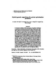
must be defined. Equation (1) gives this relationship. (1) where q (t ) is related with robot DOF and p(t ) trajectory positions. It can be computed using the IKM. However, the vector q (t ) at point i can be null if the pi (t ) is inaccessible. The DH parameters of the robot (the type of the joints, the length of its links, the joint velocity, etc.) can considerably influence the time that the robot takes to travel between two different task points. The task time between any two points is computed based on the distance travelled by robot in the operational as well as joint space. Our objective function is defined based on following notions: 1) Task points: The robot has to visit N points and then return to the initial position Easiest Way. 2) Traveling distance tour: To minimize the time of execution of the task, the minimum traveling tour of the robot visiting the N points should be found. So the minimum distance between each successive pair points should be found. This leads to know the sequence of the points giving the minimum traveled tour to achieve the task. 3) Multiplicity solutions of IKM: Each point in the operational space can be reached by multiple configurations. In this case, the optimum sequence is definitely affected by the choice of particular configuration. 4) Robot placement: The robot position has been taken into consideration because it also influences the traveled tour as well as the task time 5) Optimal solutions: The optimal accomplishment solution is based on the order of visiting the points, configuration used by the robot in each point and the relative placement of the robot and the points during the execution of this task. 6) Minimum task time: The total time of execution of the task is computed based on the displacement given by each joint between each successive task pair points and the average velocity of the robot joints. A general scenario of the objective function has been shown in fig. 1. Considering a robot has a n − DOF which has to visit N task points in 3 dimensional space. The robot can reach each point with m configurations of IKM corresponding to one of p locations. The relative position of the robot and the task is constant for all task points. Our objective is to find the tour for visiting entire task points (one by one) that should lead to have the minimum traveling time, considering the multiplicity of the robot positions and the robot configurations corresponding to each task point.

3 

1 

q relationship between the vectors (joint coordinate in joint space) and p (end-effectors coordinate in operational space)

p

configurations Using  q k m  configuration Robot configurations  regarding to each point 

dy dz

Robot possible placement in  the site 

dx

Fig. 1. Objective function

Based on the IKM of the robot in each point, the displacement of each joint q j can be calculated. Consequently we can calculate the time ti taken by the robot to travel between the point i − 1 using the configuration l th to the task point i using k th configuration corresponding to one relative location p of the robot and the task. This time is given by ⎞ ⎛ q k ji − q l j ( i −1) ⎟ p ⎜ t i = max ⎜ • ⎟ ⎜ q j ⎟⎠ ⎝ p

(2)

Where, ti p is the time between the points i and i − 1 , j = 1,2,..., n is the IKM configurations and k = 1,2,..., m is the configurations used in i points and l = 1,2,..., m is the configurations in point i − 1 . So the q k ji is the displacement of the joint j corresponding to the point i and robot position p .While r represent the IKM possible solutions. •

p q is the average velocity of the joint j . The task time tc is

N +1

tc = ∑ ti p

p

(3)

i =1

Where N + 1 corresponds to the traveling between all task points’ number and returning to the initial configuration. The general function of the optimized task time execution can be written as N +1 • ⎞ ⎛ top = min ∑ ti ⎜ j, i, k , l , q j , N , p ⎟ ⎠ i =1 ⎝

(4)

The function (4) represents the minimum time the robot takes to visit the N points (in any order, using any configuration and located on any node) and return to the initial configuration. In fact, the problem is to define the

order of the points the robot has to visit, the configuration in each point and the placement of the robot relative to these points and configuration. This consequently poses high complexity level because of dependence on multiple parameters (visited order, configuration and placement) compared to the problem proposed in [9]. The number of configurations of the robot discussed in [13] is 28 . However, this number can be reduced 2 4 if the robot has the last three axes intersected. In fact, the possible number of configurations at each point can be expired as 2m where m = 1,2,3,4 . In this case the total configurations that can be

used by the robot are (2 m ) . The possible number of order of visiting the points is N ! . While, the number of relative N

2

placements between the robot and the task is a function of number of nodes has been used to divide each length of the placement zone according to each axis [3]. So the placement number is: (5) p = xnode * ynode * znode

( )

3

number of configurations is 21 = 8 which are: 111, 112, 121, 122, 211, 212, 221 and 222. While the possible number of placements are 2 * 2 * 1 = 4 . So the total number of solution is Rsol = 3 ∗ 8 ∗ 4 = 96 . To find the optimal solution we should scan and analyze all solutions given in equation (6) which is not possible with the current computing power. In fact, the time to scan all solutions considering the minimum time for each cycle MGI equal to 35 * 10-4 second (the minimum time to evaluate the IKM with a 3.6 GHz CPU) is very huge. Considering the case of 10 task points and 8 solutions of IKM at each point and 10 nodes in each coordinate axis, the required the time to evaluate all possible solutions to find the optimal solution is 2.16*10^8 years. This time (centuries and centuries of years) was the motivation to implement the GAs in the next sections.  Y

where xnode , y node and znode are the placement number on x ,

t02 

y , z axes respectively. We should mention here that the placement zone proposed in [3] space always allows the task point accessible by the robot leading to have the IKM solution for each point at each robot position. The number of solutions is related to each robot position, visited order and number of possible configuration of the robot each point. The optimal solution should account for the three factors discussed before. Therefore, the total solution can be summarized as:

( )

Rsol = ( x node * y node * z node ) * N ! * 2 m 2

N

⎞ ⎟ ⎟⎟ ⎠4

The traveling time between B and C is ⎛ q(1,C ) 2 − q(1,B )1 q( 2,C ) 2 − q j ( 2,B )1 ⎜ , t24 = max⎜ • • ⎜ q q2 1 ⎝

⎞ ⎟ ⎟⎟ ⎠4

(7)

(8)

So the cycle time of the task becomes t c = t + t 2 . We should notice here that at each positions of the robot there is 4

a time

A

q02,B  q02,C  q01,C 

q01,A 

Position4 Position1

q02,A 

q01,B 

X

Position3  Position2 

Fig. 2. 2DOF planar robot visiting three task points in 2D space

(6)

To elaborate the objective function we present an example of the planar robot having 2 DOF which visits successively the points A, B and C. The robot can achieve the task from different position (1, 2, 3 and 4) by two different configurations at each point. If the robot uses the 2nd configuration to visit the point A and the 1st configuration to visit the points B and C, the traveling time between the points A and B is given by

⎛ q(1,B)1 − q(1, A) 2 q( 2,B)1 − q j ( 2, A) 2 ⎜ , t14 = max⎜ • • ⎜ q q2 1 ⎝

t01

B 

C

4 1

4

p

tc .

The number of possible visit order of the points is

3!/2 = 3 which are: ABC, ACB and BAC. The possible

1361

III. OPTIMIZATION BASED ON GAS We will first define the fitness function and control parameters to evaluate the optimization method. Based on these, the GAs optimization process will be stopped checking the solution convergence with respect to control parameters. A. Optimization Mechanism Description The optimization in GAs is based on natural selection of entities of chromosomes then assessment the fitness function. Each chromosome of these entities are composed of a set of entities name genes (a finite number of genes), while a set of these chromosomes constitutes a population, a set of populations known as individuals [9]. GAs requires these elements to match the Holland definition. B. Proposed Coding Problem The first step to set a GA is the choice of adequate representation to encode possible solutions of optimization problem. Each solution of the optimization problem is represented by a code which is defined by several alphabets. As mentioned before, our optimization approach considers the points visit order (1st part), the configurations in each point (2nd part), and the robot placement (3rd part). The

encoding of solutions is either by natural or by binary alphabets. Unfortunately the 1st part (points visit order) of the problem should be represented by natural encoding, because the random selection can provide the same alphabet which is not possible to consider. In this case we need a specific repairing algorithm because the input of one bit could lead to a redundant visited point in the code. However, we used the binary encoding in the 2nd and 3rd part which does not suffer from rewritten problem. Considering the example of the 2 DOF robot mentioned earlier (fig. 2) which has to visit N points with two possible configurations at each point in 2D space and assuming that the placement number equals to 4. Each chromosome (fig. 3) of the 1st and 2nd parts consists of N and N*2 genes respectively, while the third part consists of 4 genes, each pair representing the position of the robot on x and y axes. The first part consists of N numbers representing the order in which the manipulator reaches the task points. This chromosome is composed of three parts (the order of visiting the points, the IKM configuration and robot placement). The robot travels from point 5 to 3 using the configuration 2 at both points, while it finishes the task by visiting the point 2 using the first configuration. This solution is achieved from the robot position of 0 (00) on x axis and 4 (100) on y axis.

 Points visit Order  IKM solutions  Robot placement

5 3 … 2 I C2 C2 C1…C2 I Px   Py

Fig. 3. Chromosome of 2 DOF planar robot visiting N points

The general case of a n DOF robot visiting N points in 3D space containing u, v and w nodes on each coordinate axes respectively is represented in fig. 4. This figure shows a general representation of our chromosome. The robot starts from the point number 21 using the configuration number “01…1” and finishes by the point 5 using the configuration “10…1” corresponding to the robot placement of “01…1”,

 21, 3,…,5 I01...1, ...,11...0,10...1 I01...1,10…1,00…1  u        v         w

started from an initial seeded population Gas [14]. After choosing the initial population, the evaluation of this population is based on the fitness function which is the inverse of the objective function discussed in the Section II. The evaluation process consists of calculating the time corresponding to each chromosome of the population and then choosing the best solution which give the minimum time. Our regeneration operator selects chromosomes from the current population to next one. The selection of these chromosomes is based on the percentage of participation corresponding to the value of fitness function given by each chromosome in the current generation. So the chromosome having a low value of fitness function has a less chance to participate in the next population compared to one having higher fitness function value. And then a regeneration process will be applied to combine chromosomes from the current population based on its probability. The selection of the chromosome participated in the formation of the next generation is random. The crossover process in our optimization method is based on the uniform crossover [15] because it performs well compared to the two-point crossover. The used of the two-point crossover, in our chromosome, leads to generate non-homogeneous chromosomes. The control parameters of our optimization process are: the population size, the crossover rate, the mutation rate and the Elitism factor. To evaluate the proposed approach we have selected a real world industrial example of an automation plant with a 6 DOF industrial robots (Staubli RX-130 XL). The task of spot welding has been chosen because of its obvious importance during car manufacturing and other industrial plants. The coordinates of the task points are distributed on the whole virtual car’s body. The task point are defined by the vector Positions = f ( x, y, z ) where x, y and z are the coordinates of each point. The definition of x , y , z was using CAD-learning technique illustrated in [16],[17]. The deification of the task is illustrated in fig. 5. The maximum length of the occupied task zone is: 165.48mm on x axis, 30.69mm on y axis and 50.34mm on z axis. The placement part in our approach is based on a placement zone which has the length of 0.429m, 0.453m and 0.441m on x, y and z axes respectively.

Order of visit points and robot configurations  

Fig. 4. Chromosome of n DOF robot visiting N points in 3D space with u, v and w divisions on each x, y and z axes respectively

”10..1” and “00…1” nodes on x, y and z respectively. C. Optimization process The optimization process is based on the initial population generated by random selection of genes constituting its chromosomes. Moreover, the optimization process can be

1362

Fig. 5. Robotics task to evaluate the optimization approach

IV. RESULTS AND DISCUSSION In this section we have tested our optimization approach showing several results of the cycle time regarding to all used control parameters. As mentioned we have used the seeding method to improve the GAs optimization process. The percentage of participation in the seeding population enhances the random generation of the initial population. The number of seeded solutions has a trivial impact on the convergence process. The optimal time always decreases with the increase of the seeded population percentage. However, keeping in view the random selection property of the optimization process, the result showed that even with a considerable percentage in some cases, the optimum solutions are still not acceptable (60% and 80%). This may be due to the complexity of the optimization process. For all the cases having more than 50% of the seeded population, their convergence has been found in later generations with a minimum cycle time. From another point of view, this can be seen as an advantage which proves that the system is always finding new alive optimal solutions. The worst solution was 14.75sec in the 106th generation, while the best solution has been found in the generation number 176 which is more normal case with the seeded percentage of 90%. The number of convergence shows the effect of the seeded percentage e.g. it was less within seeding percentage more than it 50%, while in the case of less than 50% was higher, this is because of the compared with less than 50% case. We should mention here that the optimization process and the results are strongly related to the control parameters as well as the robot and task parameters. Comparing these results with those obtained in [9] we can clearly see the difference of the optimized interval time in this work (from 7.09 to 14.75 sec) and the optimized interval time (from 2.92 to 3.25 sec). This interval can explain the complexity of the optimization process in which in our case has more solution’s diversity.

 

100,

200,

300,

0.6, 0.7, 0.8, 0.9

...

0.1, 0.2, 0.3, 0.4

...

400

0.6 to 0.7

0.1 to 0.4

Population size

constant generation number of 110. The crossover and the mutation rates reflect the percentages of changeability of the new generated population’s chromosomes. For example if the geometrical parameter of the robot and the task are too sensitive, a law of this percentage leads to a big value of time. The worst value of 15.97sec was found within the population size of 300, the crossover rate of 0.6 and the mutation rate of 0.3. While the best solution was found in population size of 200, crossover and mutation rates of 0.7 and 0.3 respectively. These results will be considered in the next experiment.

Fig. 7. Results of the maximum and the optimal time as function of population size, crossover rate and mutation rate

Based on these results the fig. 8 shows readings of the optimization process with each new generation. The control parameters in this case were: population size of 200 with 90% of seeded solutions percentage, crossover rate of 0.7 and mutation rate of 0.3. These three parameters have given the best result (fig. 7). During the first generation, the maximum and the optimal values of the task time decreased considerably, even the maximum value was less than 45.17 sec. This can be explained due to the effect of domination of the seeded solutions.

Crossover rate

Mutation rate

Fig. 6. Experiment to test the population size corresponding to the crossover and the mutation rates

To choose the best control optimization parameters, we conducted an experimental study in which the variation of the initial population size, the mutation and the crossover rates were tested for several sets. Fig. 6 shows the tree of this experiment. First we fixed the population size to 100 and tested with the crossover rates of 0.6 to 0.9. For each crossover rate, the mutation rate was tested from 0.1 to 0.4. The same evaluation was also tested for 200, 300 and 400 generation numbers. In this case, we have considered

1363

Fig. 8. Reading of the maximum and optimal time within an optimization process

The convergence rate during all the process was found to be 38.16% in the second generation (fig. 9). This considerable value depicts that the population size, parameter of mutation and crossover rates were perfectly chosen. In fact, in the other generations the convergence rate is less than 15%.

result shows that the careful choice of the control parameters plays a trivial role to enhance the performance of the optimization algorithm. First the seeding population was evaluated to see its effect on the task time and then the control parameters’ were evaluated varying each one corresponding to its range. This provides as a great idea about the best value matching our optimization process. Results show that there are not considerably effects on the task time of inter crossover and enter mutation rates. However the mutation rate gives a best result was almost around 10%. The proposed method has reduce the computation time of the optimization process compared to the scan of all possible solutions (years) to few minutes, providing an acceptable optimal solution. REFERENCES [1]

Fig. 9. Reading of the convergence percentage within an optimization process

In fact the mutation rate of 0.1 give the best average of 11.78 sec, while the mutation rate of 0.4 gives 13.51sec of the task time. The optimization of our GAs algorithm (with generation number of 500000) leads to find an optimal time of 6.12 sec. The CPU time to find the optimal solution was 13min and 5 sec. This solution was found in the iteration number of 222857 with the following chromosome: 12, 11, 8, 9, 10, 7, 6, 5,4,2,1,3. Fig. 10 represents the final solution found by the proposed algorithm. In this figure only the visited points showed. Is we cannot predict the robot position and or the configurations of IKM of the robot. This visit order is corresponding to the configurations of 3,3,3,3,3,4,4,3,3,3,3,3 corresponding to the placement of 1,7,5 on x, y and z respectively.

Fig. 10. 3D representation of the optimal points visit order solution

V. CONCLUSION In this paper we have proposed and tested a novel optimization approach for task execution time of industrial robots based on Genetic Algorithms. Our approach takes into consideration the important factors which can effects the task’s time which are multiple configurations of the IKM of the robot and the relative placement between the robot and the task points as well as the order of visited points. The

1364

G.S. Tewolde, W. Sheng, “Robot Path Integration in Manufacturing Processes: Genetic Algorithm Versus Ant Colony Optimization”, IEEE Transactions on Systems,” Man and Cybernetics, vol. 38, no. 2, pp. 278-287, 2002. [2] E. Lawer, J. Lenstra, A. Rinnooy Kan, D. Shmoys, “The travelling salesman problem,” Chichester, UK: Wiley, 1985. [3] K. Baizid, R. Chellali, T. Bentaleb, A. Yousnaj and A. Meddahi, “Virtual Reality Based Tool for Optimal Robot Placement in Robotized Site Based on CAD’s Application Programming Interface,” Proceedings of Virtual Reality International Conference (VRIC 2010), Laval, France, April 7-9, 2010. [4] L. Abdel-Malek, Z. Li, “The application of inverse kinematics in the optimum sequencing of robot tasks,” International Journal of Production Research, vol. 28, no.1, pp. 75–90, 1990. [5] M. Dissanayake, J. Gal, “Workstation planning for redundant manipulators,” International Journal of Production Research, vol.32, no. 5, pp. 1105–18, 1994. [6] Y. Edan, T. Flash, U. Peiper, I. Schmulevich, Y. Sarig, “Nearminimum-time task planning for fruit-picking Robots,” IEEE Trans Robotic Autom, vol. 7, no. 1, 1991. [7] K. Shin, N. Mckay, “Selection of near minimum time geometric paths for robotic manipulators,” IEEE Trans Automat Control, vol.31, no. 6, pp. 501–11, 1986. [8] S. Dubowsky, T. Blubaugh, “Planning time-optimal robotic manipulator motions and work places for point-to-point tasks,” IEEE Conference on Decision and Control, Ft. Lauderdale, FL, 1985. [9] P. Th. Zacharia, N. A. Aspragathos, “Optimal Robot Task Scheduling based on Genetic Algorithms,” Robotics and Computer-Integrated Manufacturing journal, vol. 21, no.1, pp. 67-79, 2005. [10] H-S. Hwang, “An improved model for vehicle routing problem with time-constraint based on genetic algorithm,” Computers & Industrial Engineering, 42(2-4), pp. 361-369, April. 2002. [11] L. Qu, R. Sun, “A synergetic approach to genetic algorithms for solving traveling salesman problem,” Information Sciences, 117(3-4), pp. 267-283, August. 1999. [12] F. Liu, G. Zeng, “Expert Systems with Applications,” 36(3-2), pp. 6995-7001, April. 2009. [13] L. Tsai, A. Morgan, “Solving the kinematics of the most general sixand five-degree-of-freedom manipulators by continuation methods,” ASME Mechanics Conference, Boston, October 7–10, 1984. [14] S. Oman, P. Cunningham, “Using case retrieval to seed genetic algorithms,” International Journal Comput Intell Appl. , vol.1, no. 1, pp.71–82, 2001. [15] Z. Michalewitz, “Genetic algorithms+data structures=evolution programs,” 3rd ed., Berlin: Springer, 1996. [16] A. Meddahi, K. Baizid, A. Yousnadj and J. Iqbal, “API Based Graphical Simulation of Robotized Sites,” IASTED International Conference on Robotics and Applications, Cambridge, USA, pp. 485492, 2009. [17] H. Chen, W. Sheng, N. Xi, M. Song, Yifan Chen, “CAD-based automated robot trajectory planning for spray painting of free-form surfaces,” International Journal of Industrial Robot, vol.29, no. 5, pp. 426-433, 2002.