To appear in: Journal of Visualization and Computer Animation, 1995 (in press).
Genetic Programming for Articulated Figure Motion L. GRITZ and J. K. HAHN Department of EE & CS, The George Washington University, 801 22nd Street NW, Room T-624, Washington, DC 20052, U.S.A. email:
[email protected] SUMMARY We present an approach to articulated figure motion in which motion tasks are defined in terms of goals and ratings. The agents are dynamically-controlled robots whose behavior is determined by robotic controller programs. The controller programs for the robots are evaluated at each time step to yield torque values which drive the dynamic simulation of the motion. We use the AI technique of Genetic Programming (GP) to automatically derive control programs for the agents which achieve the goals. This type of motion specification is an alternative to key framing which allows a highly automated, learning-based approach to generation of motion. This method of motion control is very general (it can be applied to any type of motion), yet it allows for specifications of the types of specific motion which are desired for a high quality animation. We show that complex, specific, physically plausible, and aesthetically appealing motion can be generated using these methods. KEY WORDS: Computer animation Genetic Programming
Evolutionary Computation
Learning
Robotics
INTRODUCTION The tradeoff between control and automation is a well known problem in computer assisted character animation. It has been the goal of many researchers to allow automation of agents while still maintaining control. Despite this, most professionals still use key framing because most of the automatic motion control schemes have not allowed for sufficiently specific control over the agents. This is a laborious and tedious process for those professionals, and high quality motion is often difficult to achieve even for skilled animators. We propose a new technique for animating articulated figures which highly automates the animation process, is extremely general (can be used for a variety of motion tasks), yet allows the user to be quite specific about what motion is to be generated. We find that humans may not know how to specify good motion, but we can easily recognize good or bad motion when we see it. Our technique is well adapted to these strengths and weaknesses. The guiding principle is: let the system generate the motion, and let the human provide the determination of what is “good.” Our method employs the AI technique of Genetic Programming (GP). Our GP technique can be thought of from several perspectives: 1. Our agents are dynamic robots whose actions are determined by controller programs. GP allows us to find a controller program for the action we want the agent to perform. 2. The animator does not need to provide the controller programs, only a metric of what motion is good. We suspected that it may be easier to quantify (rate) motion after the fact than to generate the description of the motion itself. This turned out to often be the case, particularly for people who are not professional animators. 3. The process of developing controller programs could be thought of as a learning process or a planning process. A surprising number of interesting motion control problems can be stated as problems of program induction. That is, we know that the solution to the problem is an appropriate formula or computer program, but we are not sure how to write the program. GP allows us to find the appropriate controller program for our agents to achieve their goals.
RELATED WORK Witkin and Kass [1] proposed the spacetime constraints method of automatically generating motion (later enhanced by Cohen [2]). Their goal was to see how many of the principles of animation outlined by Lasseter [3] could be derived automatically from first principles. Spacetime constraints generates kinematic motion which both satisfies high level goals (e.g. “jump from here to there”) and also appears to be physically plausible. The resulting motion also tended to exhibit many of the principles of traditional animation (e.g. squash and stretch, anticipation, follow-through). The method involves optimizing the kinematic positions of the articulated figure, using energy consumption as an objective function and constraining the solution in order to ensure that the motion is physically plausible. Unfortunately, this method suffers from several drawbacks: it can be numerically unstable and its solution depends on the initial guess provided to the optimizer, the solution can easily be a local minimum, energy may not be the best criteria to optimize, and the method appears to need a significant amount of hard-coding and mathematical sophistication to use. More recently, other researchers proposed methods of automatically generating walking motion using search and optimization techniques [4,5]. Both gave impressive results, yielding physically plausible motion and automatically finding a number of walking methods. However, the resulting motion had high specialization (i.e. they made walking gaits, not general motion), but low specificity (i.e. they both simply walked forward, rather than having more specific instructions, like “walk to position X”). Both of these methods were optimizing structures of fixed complexity (a network of fixed topology and a stimulus-response table, respectively). We believe that this is a disadvantage. We chose a different representation, namely a mathematical description (computer program) describing how the joint forces vary with time and changes in the state of the simulation. We believe that this representation offers many advantages. Such a representation is appropriately optimized using the GP technique. It is also interesting to note the work of Karl Sims, who used a GP-like process to evolve procedural textures, where the fitness metric was human evaluation [6]. Sims also wrote a paper describing the use of evolutionary programming to design entire creatures [7], in which even the creature topology was evolved for walking, swimming, etc. In contrast, our work deals with figures of fixed topology and geometric structure, as one would expect for character animation.
GENETIC PROGRAMMING Genetic Programming (GP)[8] is an evolutionary metaphor similar to Genetic Algorithms (GA) [9,10,11]. The major difference is that GA’s usually operate on fixed length binary strings, while GP operates on computer programs of varying complexity. One advantage to this approach is that often the complexity of an optimal solution to a problem is not known a priori. With GA, the complexity (length of the binary strings) must be specified at the start. On the other hand, GP can evolve a complexity level appropriate to the problem. The basic GP algorithm is simple and may be explained very briefly. We have a particular optimization problem, the solution of which is a computer program. Though we could operate on any programming language representation, for simplicity we operate on program parse trees. These parse trees can be represented by LISP S-expressions [12]. Figure 1 shows a typical parse tree and its associated Sexpression. The parse tree and S-expression correspond to the following formula in algebraic notation: x2 + (y - 3.27)
2
+ *
x
-
x
y
3.27
(+ (* x x) (- y 3.27)) Figure 1: A parse tree and corresponding S-expression.
Note that the parse tree consists of a root node (which may optionally be a special function such as a list), functions with one or more arguments, and terminals (leaves of the tree) which are either numerical constants, named variables, or functions which take no arguments. The GP paradigm requires the following problem-dependent inputs: 1. A set of terminals (constants and named variables) and a set of functions, out of which the parse trees can be generated. 2. A fitness function, which returns a measure of the performance of an arbitrary individual program. 3. A termination criteria, which recognizes when it has come across an individual program which adequately solves the problem at hand. 4. The number of individuals in the population (M), the maximum number of generations to calculate (G), and other miscellaneous variables which control the workings of the GP run. For the first generation, we start with a population of randomly generated individuals (programs), and use the fitness function to rate their performance. We should expect that the fitness values of these random individuals will be quite low, since the chances are slim that a random computer program will solve our problem exactly. We form the populations of subsequent generations using genetic operators: a) Reproduction, which copies (without alteration) individuals from the previous generation that had high fitness values. b) Crossover, which combines two individuals from the previous generation to yield two new individuals. This is typically done by swapping randomly chosen subtrees of the two programs (see figure 2). c) Mutation, which replaces a randomly selected subtree with a new randomly generated subtree. Since the individuals involved in these operations are typically selected in some type of fitness-proportionate manner, unfit individuals will tend not to make it to the next generation while highly fit individuals will tend to survive. The alterations resulting from crossover will sometimes result in individual programs which are more fit than any programs seen in previous generations.
3
*
+ *
3.14
+
x
+
abs
y
8
x
+
y
y
y (* 3.14 (+ y 8))
x
-
abs
(+ x (- x (abs y) ))
(* (abs y) (+ y 8))
8
x
3.14
(+ x (- x 3.14 ))
Figure 2 (a) Parse trees before crossover (left side). The bold regions denote the subtrees selected for crossover. (b) The resulting parse trees after crossover (right side).
This cycle is repeated for each generation until a maximum number of generations is reached, or until an individual is found which adequately solves the problem at hand (i.e. meets the termination criteria). Each generation tends to have individuals with higher fitness than the previous generation, and this often results in finding optimal individuals which could not have been found by blind random search. The highest level of the GP algorithm can be formalized as below: let M = population size; let G = maximum number of generations to run; create M random programs for generation 1; for gen = 1 to G do: for i = 1 to M do: fi = fitness of individual i; if individual i solves the problem adequately, then terminate; endfor; construct generation gen+1 using reproduction, crossover, mutation; endfor; report the best individual found.
Since the Genetic Programming paradigm is driven by stochastic processes such as the initial population of random programs and the probabilistic selection of individuals for reproduction and crossover, it is not guaranteed that a solution to our problem will be solved in any particular run. However, we can perform multiple independent runs (with different random number seeds on each run) until we find a solution that is adequate.
SYSTEM OVERVIEW The conceptual layout of our system is shown in Figure 3. From the perspective of the animator, the GP and dynamics subsystems may be treated as black boxes.
4
Output
controller program
Articulated figure dynamics simulation
GP System
fitness metric
Input/Output of System
System (black box)
Input (supplied by user)
figure model
Figure 3: Structure of the system
For any given animation, the system needs to understand the dynamics of any articulated figures or other agents involved in the simulation. This information must be supplied for the dynamics to be computed properly. The figure model includes connectivity of the figure; geometry, masses, and inertias of the various links; and descriptions of the capabilities of the figure (e.g., joint limits, force and torque ranges for the “muscles”, pressure sensors). This information generally does not change over the course of an entire animation. For each motion sequence, the animator must supply a fitness metric; in other words, a formula which will rate a motion sequence. The rating should be a low number if a prospective motion sequence is close to that wanted by the user, a higher number if it deviates from the goals. The nature of the fitness metric is discussed in later in this paper. When a GP run has finished, the final output of the GP subsystem is a single controller program. This controller program is the one which, when used to govern the actions of a simulated agent, resulted in the best rated agent according to the user-supplied fitness metric. This controller program may then be used to generate the motion control needed for the animation. Dynamics Subsystem The dynamic system simulates the physics of articulated bodies. We use the dynamics methods outlined in [13,14,15] to model articulated figures as trees of rigid links. Each joint is controlled internally by a damped angular spring. The joint has a “neutral” (or desired) orientation. The spring pushes the joint toward the desired orientation with a torque proportional to the angle between the actual and desired orientations (figure 4). This is called a proportional derivative (PD) controller, and is a common technique used in both computer animation and robotic control. .
τ i = k1 θ i + k2 θ i Rigid Link i+1 (actual position)
Rigid Link i θ desired position of link i +1
Joint j (3 deg. of freedom) Figure 4: Torque at a joint is proportional to the angular difference between actual and desired orientations of the links (desired angle is the output of the controller program).
At each time step in the integration, the robotic controller program is evaluated. The controller program is interpreted as a list of the desired orientation angles for the joints. The differences between these desired angles and the actual angles yield the torques and forces which drive the figure. Because the
5
system is based on dynamics and performs collision detection and response, we are guaranteed to have resulting motion which appears physically plausible. Simulation of a motion sequence for controller C: t = 0; while t < time_limit do: evaluate controller C, yielding desired joint angles α1...αn. integrate dynamics forward for time δt; t = t + δt; endwhile;
GP Subsystem The GP subsystem runs the basic GP algorithm described earlier. Whenever it is time to evaluate the fitness of an individual, the dynamics subsystem is invoked to simulate the situation, given the particular individual as the robot controlling program. When the simulation is over, the user-supplied fitness evaluation function rates the performance based on statistics collected by the dynamics program. Earlier we alluded to the notion that the GP system needs an appropriate set of functions and terminals (parse tree leaves) out of which it constructs the controller programs. To a large extent this is customizable, but requires some careful judgment. We do not want terminals and functions which are not needed to solve the problem, since they will only slow down our search for the correct solution. On the other hand, if a particular problem’s unknown solution requires a function which is not in our set, we will never find the correct solution. In short, we want a minimal set of basis functions which will allow the controller to perform its duties. The functions in the parse trees should minimally consist of basic arithmetic functions (+, -, *, %).1 We also found it critical to include the operator ifltz, which takes three subtrees as arguments: if the first evaluates to a value less than 0, then evaluate and return the second subtree, else evaluate and return the third subtree. We consider this set of primitives to be minimal, but sufficient. For certain models or motion tasks, it may be advantageous to add more mathematical functions (such as cos, which could aid in generation of internal oscillators, or abs), control functions (such as while), functions specific to the model or task at hand (such as distance-to-nearest-obstacle), or functions which produce side effects when evaluated (such as release-grip). Which functions to add depends largely upon what functionality is built into the models being controlled and the intuition of the designer when considering the particular motion tasks. The terminals in the controller programs correspond to the internal state variables of the agent and the outputs of any sensors accessible to the agent. For example, there may be terminals (named variables) which correspond to the agent’s position, velocity, joint angles, external forces on its limbs, etc. The terminals look up the sensor outputs or state variables when they are evaluated. In other words, the variables are continually updated by the dynamics subsystem therefore they contain different values when the controller is evaluated at each integration step. It is also possible to have variables contain the status of subgoals (e.g. one variable may become nonzero when a subgoal is met, allowing if-then statements in the controller program to switch behaviors at that point). In addition to named variables, it is useful to have numerical constants. Since we do not know beforehand what constants might be useful, we simply sprinkle the initial random population's parse trees with randomly chosen floating point values. This is a well known GP technique called use of the ephemeral random constant, and is described in detail in [8]. 1
% indicates protected division which is identical to / but does not cause an exception upon division by zero.
6
The structure of the controller program naturally reflects the model and task at hand. In the case where we want torque values at all joints, the root nodes of the parse trees will all be lists whose length is the number of degrees of freedom controllable by the agent. Each element in the list is a controller program for that particular degree of freedom (figure 5). When this is the case, the trees are constrained to have this topology—the original random trees are all lists, and the crossover operation is guaranteed not to disturb this structure. Thus, each evolved program actually consists of mini-programs for controlling each joint.
Controller = (list (expr1) (expr2) (expr3) (expr4) (expr5))
1 dof 1 dof 3 dof
Figure 5: Controller programs are lists giving mini-control programs for each degree of freedom in the agent.
These mini-programs for the joints are evaluated independently, but since they are built of primitives which may consist of state variables of the agent, the controller programs for different joints may produce coupled actions. The nature of the GP paradigm tends to produce coupled motion when advantageous and independent motion when that approach is more productive. This is why the lack of externally imposed structure on the controller solution works to our advantage—the GP will naturally evolve a solution structure appropriate to the problem being solved.
CONSTRUCTING FITNESS MEASURES Once the system understands the dynamics and capabilities of the agent, it can run the dynamics simulations. The GP subsystem generates controller programs which are potential solutions to the motion control problem at hand. These controller programs are passed one at a time to the fitness function, which is responsible for generating a rating for that controller. The fitness function uses the dynamics system to simulate the motion using that particular controller program, then uses statistics supplied by the dynamics system to compute a fitness rating. Evaluate fitness of controller C: Simulate the motion using controller C; fit = main_goal + style_points; return fit;
When generating actual motion, a good fitness metric that results in the motion we are seeking can be specified using an astonishingly small amount of code. Conceptually, we divide the fitness measure into a main goal and style points. The main goal should be a simple metric of whether the primary task of that motion sequence has been fulfilled. For example, if the point of the motion sequence is to move the figure to the “X”, then the main goal should simply be the distance between the figure and the “X” at the end of the time allotment (remember that lower numbers correspond to better performance).
7
Since the motion is so grossly underconstrained, the GP system can often find outrageous ways of meeting such a simple fitness requirement. For example, it might somersault to the goal point instead of hopping. Because of this, we find it useful to add style points, which can be thought of as additional rewards or penalties granted to the individual’s performance. Examples of style points include: 1. Penalties for hitting obstacles or violating safety rules (“don’t hit your head on the floor”). 2. Rewards for performing the action quickly, or slowly. 3. Penalties for inefficient behavior (such as taking the long way around an obstacle or sitting for a long time, then rushing when it gets close to the time limit). 4. Rewards for ending in “neutral positions” and remaining in control (you don’t want the actor tangled up or laid across the floor when he completes his action). 5. Rewards for minimizing energy consumption are useful at times. Most of the time, however, we found that this did not improve the quality of motion in any significant way. Even when energy considerations were useful, the effects tended to be very subtle, and not as important as the other style considerations. 6. Problem-dependent terms (e.g., whether certain subgoals were met). The following section will clarify the role of these terms in the fitness function by discussing specific examples.
RESULTS Luxo revisited Our first example returns us to the desk lamp. This seems appropriate since the film Luxo, Jr. [16], though completely key framed (thus dependent on the exhausting labor of a highly skilled animator), is still considered the pinnacle of computer animation quality. We wanted to teach the lamp to be able to move about. It would not have been considered a success to simply move forward—we wanted to generate a controller program to bring it to rest on a particular spot, to show that we could perform any intricate scripted motion we desired. Our lamp model was a fully 3-dimensional articulated body with 4 links and 3 internally controllable degrees of freedom. All dynamics were simulated in 3-D. The geometry, masses, inertias, and so on were given to the system. The lamp had access to its position relative to the goal point, its velocity, and the amount of force being imparted to its base through contact with the floor. The set of terminals consisted of those state variables described above, time, and a random selection of floating point constants. The function set consisted only of { +, -, *, %, ifltz }. These choices were suggested by prior GP research, especially [8]. We experimented with several fitness measurements. The one that we found most successful was a blend of the following constraints: 1. Main goal: distance between base center and goal point “X” at the end of the time allotment. 2. Style points: a weighted sum of the following: a) bonus for completing the motion early (how much time did it take to get to the “X”). b) penalty for excess movement after goal was met (this was to keep it still after it got done). c) penalty for hitting its head or falling over. d) bonus for ending with joints at neutral angles. The formula which computed this fitness metric (given access to statistics computed by the dynamics subsystem) was surprisingly small—about a half dozen lines of C code. We found that immediately placing all of the style considerations on the motion did not give the GP process the best opportunity to discover fit individuals, simply because it was so restrictive. We solved this problem by rating controller programs based on the main goal only for the first few generations. Then
8
we slowly phased in the style considerations, generation by generation. The effect was to teach it how to get to the “X” first, without regard to whether it fell over afterward or whether it ended in a neutral position. Once it had mastered that task, then we placed more and more restrictions on it. By the time we got to the 50th generation, the motion included the full set of style considerations. In this manner, we allowed the motion to start crudely and get progressively more stable over several generations. This was easier for the system than requiring optimal motion at the very start. In this example, we ran the GP system for 50 generations using a population of 250 individuals. For each new generation, 90% of the new individual programs were generated using crossover, and the remaining 10% were generated using reproduction. We did not use mutation for the examples described in this paper because it was found not to be significant compared to crossover. These parameters are suggested in [8], and our experiments indicate that the results were not particularly sensitive to changes in these values. The resulting controller program produced a hopping motion which brought the lamp to the exact spot we desired (see Figure 6). The motion appeared smooth, physically realistic, efficient, and surprisingly organic. Note that the solution involved two hops. A solution with such severe discontinuities (such as collisions) would not be found by a local gradient-based optimization method such as spacetime constraints. Figure 7 shows a sample controller program which made a successful jump. The controller programs are usually opaque to human interpretation, but we are generally not concerned with the robot’s internal mechanisms for movement.
Figure 6: Lamp’s Jumping motion. The primary task is to locomote to the target point, shown by the “X”. Note that the resulting motion brings the lamp to the specific target point desired, illustrating a high level of control. (list (- (ifltz a0 pz a2) (% a1 t)) (ifltz (- (- (ifltz a0 pz a2) (% a1 t)) (ifltz (+ a2 15.4963) (ifltz a0 pz a2) (% a1 a2))) (ifltz (% (- s0 vx) (+ a2 s0)) (% (- s0 vx) (+ a2 s0)) (+ (- a1 a1) (- a1 t))) (% (+ a1 vz) (ifltz (* pz a1) (% a0 pz) (% px a0)))) (- (ifltz s0 (ifltz (- (% vx a0) (% vx vx)) (- (% vx a0) (- (+ -28.4382 t) (% a1 t))) (* 16.5266 s0)) vz) (+ a1 vz)))
Figure 7: Sample successful controller program. The named variables correspond to angle, force, position, and velocity sensors. The resulting programs are generally not easy for humans to interpret.
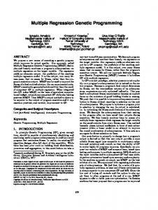
It is particularly enlightening to view the progress being made in the learning process, generation by generation. If one views the motion sequences of the best individual of each generation, it is easy to believe that a single lamp is actually learning how to locomote by trial and error. After we evolved controller programs to enable the lamp to locomote, we wanted to see how well the system could handle obstacles and other severely constraining conditions. We decided to teach the lamp how to limbo. Using the genetic system with a single additional style term—a large penalty for hitting his head on the limbo pole—we were able to produce a series of motions for various heights of the limbo pole. These motions were used to make the animated short film, “L*xo Learns to Limbo.” The resulting motion was very convincing. Because the motion had slight imperfections and at times incorporated seemingly “clever” strategies, it appeared organic rather than robotic (see figures 8 and 10).
9
Figure 8: The lamp can learn to avoid obstacles when additional constraints are added to the system.
Humanoid Figure The next test was intended to see if this paradigm could scale up to models with many degrees of freedom. We modeled an articulated humanoid figure and taught it to do a variety of simple tasks. The figure had a total of 28 degrees of freedom. Between 4 and 10 degrees of freedom were controlled by the genetic controllers at any one time, depending on the motion task (the others were under simple dynamic control). For the genetic programming step, we left the function set as before: { +, -, *, %, ifltz }. The terminal set was expanded to include all internal joint angles, force sensors, and positions of end effectors. Depending on the motion task, we used genetic runs of between 20 and 50 generations, each comprised of between 100 and 400 individual controller programs.
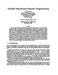
Figure 9: Herman learns a variety of tasks. (a) touching/grasping targets; (b) gesturing/touching his nose
Using similar goals and style points as described before, we were able to train the humanoid to perform a number of simple, but nontrivial, motion tasks. These included pointing, gesturing, and touching objects or parts of its body. Figure 9 shows some sequences of these learned motions.
DISCUSSION We propose the following guidelines for determining whether our system is successful: 1. Can it generate complex, general motion?
10
2. Does the animator retain enough control to easily generate motion for specific tasks? 3. Is the motion physically plausible? (Physically implausible motion distracts the viewer.) 4. Does the motion have appeal? (e.g. does it look organic? Can one imagine emotional content?) We believe that our technique satisfies all of these criteria in generating a variety of motion tasks. In no way is it hard coded for a particular type of motion, yet it is able to generate motion which matches our specific goals. All of the motion is both physically based and biologically believable for the construction of our agents. Finally, the resulting motion sequences pass the hardest test: it is entertaining to watch. The “L*xo Learns to Limbo” video is a prime example. The motion is fluid and believable, and was constructed using a fitness metric of less than a dozen lines of C code. We feel that this was a more efficient method (for this task) than key framing. While the development of good fitness metrics is a skill in itself, we found that it was a much easier skill to develop than motion specification. While the first fitness metrics we used were developed through trial and error, we found that subsequent fitness metrics for different tasks and models were substantially similar, and needed very little tweaking for different motion tasks. We admit that the choices for fitness metrics and the function and terminal sets were somewhat ad-hoc. Our continuing research addresses the issue of exactly which fitness measures are best, which members of the function and terminal sets are essential, and how the choice of these parameters affects the efficiency of the learning. The learning process takes time proportional to the number of generations (G) and number of individuals per generation (M), the amount of time to simulate for each trial, and the accuracy of the integration. This is because each individual controller program must be evaluated by simulation of the dynamics. Even if the simulation can be calculated faster than real time, it still must be performed for roughly M×G different individuals. For our examples, computation time was on the order of a few minutes per generation on a MIPS R4000 processor. Though this may not be a particularly fast technique in terms of CPU time, it was quite efficient in human animator time. In addition, the GP algorithm easily lends itself to massive MIMD parallelization, since the simulation and evaluation of each individual controller program can be performed independently. We are currently exploring such a parallelization scheme. A clear deficiency in the scheme is the “brittleness” of the resulting controller programs. The learning process produces a controller for a particular task, rather than a general skill, and the controller is sensitive to initial conditions. We are currently exploring ways to make more “robust” controllers. We have just begun work in this promising area. There are many possible extensions to this work, including putting an intuitive interface around the package which will allow automatic construction and tuning of fitness metrics, evolving more robust controller programs for complex tasks such as walking on uneven terrain with obstacles, and building libraries and hierarchies of controller programs. We also would like to explore the relationship between key framing and automatic motion generation. Clearly it is not an either-or situation. Key frames may be used as hints or constraints for the automatic motion generation, or automatic motion may be used as a starting point for key framing. In addition, we suspect it will be advantageous to have some degrees of freedom for a figure generated automatically, while others are key framed. ACKNOWLEDGMENTS
This work was partially supported by NASA GSFC (NCC 5-43). We would also like to thank the other members of the GWU Graphics Lab for their helpful discussions and reviews. REFERENCES [1]
Witkin, Andrew and Michael Kass. Spacetime Constraints, Computer Graphics, 22(4):159-168, August 1988.
11
[2] [3] [4] [5] [6] [7] [8] [9] [10] [11] [12] [13]
Cohen, Michael F. “Interactive spacetime control for animation,” Computer Graphics, 26(2):293-302, July 1992. Lasseter, John. “Principles of traditional animation applied to 3D computer animation.” Computer Graphics 21 (Proceedings of Siggraph ’87), pp. 35-44. Ngo, J. Thomas and Joe Marks. “Spacetime Constraints Revisited,” Proceedings of Siggraph ’93, pp. 343350. van de Panne, Michiel and Eugene Fiume. “Sensor-actuator networks,” Proceedings of Siggraph ’93, pp. 335-342. Sims, Karl. Artificial evolution for computer graphics. Computer Graphics, 25(4):319-328, 1991. Sims, Karl. Evolving Virtual Creatures, Computer Graphics Proceedings, Annual Conference Series 1994 (Proceedings of SIGGRAPH ‘94), pp. 15-22. Koza, John R. Genetic Programming. MIT Press, 1992. Goldberg, David E. Genetic Algorithms in Search, Optimization, and Machine Learning. AddisonWesley, 1989. Davidor, Yuval. Genetic Algorithms and Robotics: A Heuristic Strategy for Optimization. World Scientific, 1991. Davis, Lawrence, ed. Handbook of Genetic Algorithms. Van Nostrand Reinhold, 1991. Steele, G. Common Lisp, The Language. Digital Press, 1984. Armstrong, William W. and Mark W. Green. “The dynamics of articulated rigid bodies for purposes of animation,” Visual Computer Springer-Verlag, 1985, pp. 231-240.
[14] Hahn, James K. “Realistic animation of rigid bodies,” Computer Graphics, 22(4):299-308, August 1988. [15] Wilhelms, Jane. “Dynamics for Computer Graphics: a Tutorial,” Siggraph ‘90 Course notes #8 (Human Figure Animation: Approaches and Applications), pp. 85-115. [16] Pixar. Luxo, Jr. (computer animated film), 1986.
Figure 10: L*xo Learns to Limbo
12