Geometry and Attribute Compression for Voxel ... - Semantic Scholar
Recommend Documents
the manufacturing, architectural, and entertainment indus- tries for visualizing 3D data, ... Topological Surgery (TS) scheme 45, the first connectivity- preserving ...
other point of view, complete 3D geometry reconstruc- tion is not presently ... image and Euclidean geometry of those points, deter- mination of projective ...
Then, we call the tradi- .... The point of view was set at center of three ... sion (ICCV'98), Bombay, India, pp. ... âAppearance-Based Virtual View Generation of.
our method is free since only the prediction weights have to be modified in the code. .... this vertex (Average Parallelogram Prediction or APP), as- ..... We call Ï2.
maps the formal parameters n and x to register 1, and register pair 2 and 3, respectively. .... domain-specific product parameters such as product type, spec class, product dimension and ... block of spec text. These extractions are cheap.
Wallflower [5]. Silhouettes are used and we extract linguistic summarizations of human state based on crisp voxel person and fuzzy logic [1]. The resulting ...
carried out on attribute reduction [2], particularly by people in the Rough Sets society. ... plastic heavy black small t3 round wood heavy white large t4 round wood light white ... cation of elements of the universe as the whole set of attributes.
Abstract. Filtered Attribute Subspace based Bagging with Injected. Randomness (FASBIR) is a recently proposed algorithm for ensembles of k-nn classifiers [28].
Software Engineering Institute. Carnegie ... to accomplish is to document the attribute primitives in a consistent fashion. Product lines ... to the design task but does not remove the necessity for designing to achieve all of the normal quality ....
James Clark has provided a derivative-based validation algorithm for handling such interdependencies. This paper shows another algorithm, which is based on ...
Matthew G. Richards,* Adam M. Ross,â David B. Stein,â¡ and Daniel E. Hastings§. Massachusetts ... (c) 2009 M.G. Richards, A.M. Ross, and D.E. Hastings ..... concept enhancements design variables (units) a tm o s p h e ric d ra g flu c tu a tio n.
GEOMETRY AND PROOF. A report based on the meeting at Manchester Metropolitan University, 3 rd. March 2001. Keith Jones and Melissa Rodd. University of ...
Key words and phrases: Nearest-neighbor, distance function, classification, ... Because predictors may be either categorical or continuous, a good distance func-.
Randeep Bhatia and Sudipto Guha and Samir Khuller and Yoram J. Suss- mann. Facility Location with Dynamic Distance Functions. J. of Combinatorial.
GEOMETRY-ADAPTIVE DATA COMPRESSION FOR TDOA/FDOA LOCATION. Mo Chen and Mark L. ... to compress the data using a wavelet packet transform and show ..... performance, no entropy coding is applied after quantization. .... Acoustics,. Speech, and Signal
email: [email protected]. Xiaolin Wu ... description coding, networked 3D graphics, quality of ser- ... ity of multi-resolution geometry coding supports streaming.
under the guidance of the proximate record graph. Exten- ... Graph, Semi-supervised Learning ..... ted to Google API to retrieve relevant documents, and the.
$alpha and $sigma attributes can be stored in stacks (however $epsilon and $phi have to be hooked in the tree itself). On the other hand, the incremental ...
Jun 3, 2016 - We use the terms speech compression, speech coding, and ...... Tremain, T.E. The government standard linear predictive coding algorithm: ...
parate field data, with more points sampled in regions con- taining more ... nectivity information, such as point clouds, which are be- ... Devillers and Gan-.
Oct 19, 2011 - Editor: Hans P. Op de Beeck, University of Leuven, Belgium. Received April 8, 2011; Accepted ..... Hans Huber. 11. Schelling D, Schächtele B ...
Simulated Alzheimer's Disease. Gerard R. Ridgwaya, Oscar Camaraa, Rachael I. Scahillb, William R. Cruma,. Brandon Whitcherc, Nick C. Foxb, and Derek L. G. ...
May 10, 1997 - [LaBerge, 1994]. Gravity studies first revealed the MCR ..... the air gun source strength is known, slight variations in the source and energy ...
Geometry and Attribute Compression for Voxel ... - Semantic Scholar
ometry (tree and plants in the San Miguel scene); and a 3D model obtained from real-life photographs using ..... Tech. rep., NVIDIA Corporation, 2010. 1, 8, 9.
EUROGRAPHICS 2016 / J. Jorge and M. Lin (Guest Editors)
Volume 35 (2016), Number 2
Geometry and Attribute Compression for Voxel Scenes Bas Dado, Timothy R. Kol† , Pablo Bauszat‡ , Jean-Marc Thiery and Elmar Eisemann§ Delft University of Technology
Figure 1: Compressed voxelized scene at different levels of detail, rendered in real time using raytracing only. Our hierarchy encodes geometry and quantized colors at a resolution of 128K 3 . Despite containing 18.4 billion colored nodes, it is stored entirely on the GPU, requiring 7.63 GB of memory using our compression schemes. Only at the scale shown in the right bottom image the voxels become apparent. Abstract Voxel-based approaches are today’s standard to encode volume data. Recently, directed acyclic graphs (DAGs) were successfully used for compressing sparse voxel scenes as well, but they are restricted to a single bit of (geometry) information per voxel. We present a method to compress arbitrary data, such as colors, normals, or reflectance information. By decoupling geometry and voxel data via a novel mapping scheme, we are able to apply the DAG principle to encode the topology, while using a palette-based compression for the voxel attributes, leading to a drastic memory reduction. Our method outperforms existing state-of-the-art techniques and is well-suited for GPU architectures. We achieve real-time performance on commodity hardware for colored scenes with up to 17 hierarchical levels (a 128K 3 voxel resolution), which are stored fully in core. Categories and Subject Descriptors (according to ACM CCS): I.3.3 [Computer Graphics]: Picture/Image Generation—Display algorithms I.3.7 [Computer Graphics]: Three-Dimensional Graphics and Realism—Raytracing
1. Introduction With the increase of complexity in virtual scenes, alternative representations, which enable small-scale details and efficient advanced lighting, have received a renewed interest in computer graphics [LK10]. Voxel-based approaches encode scenes in a highresolution grid. While they can represent complicated structures, † [email protected] ‡ [email protected] § [email protected] c 2016 The Author(s)
c 2016 The Eurographics Association and John Computer Graphics Forum Wiley & Sons Ltd. Published by John Wiley & Sons Ltd.
the memory cost grows quickly. Fortunately, most scenes are sparse – i.e., many voxels are empty. For instance, Fig. 1 shows a scene represented by a voxel grid of 2.25 quadrillion voxels (128K 3 ), but 99.999% are actually empty. Although hierarchical representations like sparse voxel octrees (SVOs) [JT80, Mea82] exploit this sparsity, they can only be moderately successful; a large volume like the one in Fig. 1 still contains over 18 billion filled voxels. For large volumes, specialized out-of-core techniques and compression mechanisms have been proposed, which often result in additional performance costs [BRGIG∗ 14]. Only recently, directed
B. Dado, T. R. Kol, P. Bauszat, J.-M. Thiery & E. Eisemann / Geometry and Attribute Compression for Voxel Scenes
acyclic graphs (DAGs) have shown that even large-scale scenes can be kept entirely in memory while being efficiently traversable. They achieve high compression rates of an SVO representation with a single bit of information per leaf node [KSA13]. Their key insight is to merge equal subtrees, which is particularly successful if scenes exhibit geometric repetition. Unfortunately, extending the information beyond one bit (e.g., to store material properties) is challenging, as it reduces the amount of similar subtrees drastically. Our contribution is to associate attributes to the DAG representation, which are compressed separately while maintaining efficiency in rendering tasks. To this extent, we introduce a decoupling of voxel attributes from the topology and a subsequent compression of these attributes. Hereby, we can profit from the full DAG compression scheme for the geometry and handle attributes separately. Although the compression gain is significant, the representation can still be efficiently queried. In practice, our approach enables realtime rendering of colored voxel scenes with a 128K 3 resolution in full HD on commodity hardware while keeping all data in core. Additionally, attributes like normals or reflectance can be encoded, enabling complex visual effects (e.g., specular reflections). Our main contributions are the decoupling of geometry and voxel data, as well as the palette compression of quantized attributes, delivering drastic memory gains and ensuring efficient rendering. Using our standard settings, high-resolution colored scenes as in Fig. 1 require on average well below one byte per voxel. 2. Related work We only focus on the most related methods and refer to a recent survey by Balsa Rodríguez et al. [BRGIG∗ 14] for other compression techniques, particularly for GPU-based volume rendering. Large datasets can be handled via streaming; recent approaches adapt a reduced representation on the GPU by taking the ray traversals through the voxel grid into account [GMIG08, CNLE09, CNSE10]. Nonetheless, transfer and potential disk access make these methods less suited for high-performance applications. Here, it is advantageous to keep a full representation in GPU memory, for which a compact data structure is of high importance. Dense volume compression has received wide attention in several areas – e.g., in medical visualization [GWGS02]. These solutions mostly exploit local coherence in the data. We also rely on this insight for attribute compression, but existing solutions are less suitable for sparse environments. In this context, besides SVOs [JT80, Mea82], perfect spatial hashing can render a sparse volume compact by means of dense hash and offset tables [LH06]. While these methods support efficient random access, exploiting only sparsity is insufficient to compress high-resolution scenes. Efficient sparse voxel octrees (ESVOs) observe that scene geometry can generally be represented well using a contour encoding [LK11]. Using contours allows early culling of the tree structure if the contour fits the original geometry well, but this can limit the attribute resolution (e.g., color). While it is possible to reduce the use of contours in selected areas, this choice also impacts the compression effectiveness drastically. Voxel attributes are compressed using a block-based DXT scheme, requiring one byte for
colors and two bytes for normals per voxel on average. For highresolution scenes, a streaming mechanism is presented. Recently, Kämpe et al. observed that besides sparsity, geometric redundancy in voxel scenes is common. They proposed to merge equal subtrees in an SVO, resulting in a directed acyclic graph (DAG) [KSA13]. The compression rates are significant and the method was even used for shadow mapping [SKOA14, KSA15]. Nonetheless, the employed pointers to encode the structure of the DAG can become a critical bottleneck. Pointerless SVOs (PSVOs) [SK06] completely remove pointer overhead and are wellsuited for offline storage. However, they do not support random access and cannot be extended to DAGs, as PSVOs require a fixed, sequential memory layout of nodes. While several reduction techniques for pointers have been proposed [LK11,LH07], they are typically not applicable to the DAG. These methods assume that pointers can be replaced by small offsets, but in a DAG, a node’s children are not in order but scattered over different subtrees. Concurrent work presented a pointer entropy encoding and symmetry-based compression for DAGs, but does not support attributes [JMG16]. Adding voxel data reduces the probability of equal subtrees, making DAGs unsuitable for colored scenes. The recently proposed Moxel DAGs [Wil15] address this problem. In every node, they store the number of empty leaf voxels (assuming a complete grid) in the first child’s subtree. During traversal, two running sums are kept – the number of empty leaves and total leaves – to compute a sequential unique index for every existing leaf voxel, with which the corresponding attributes are retrieved from a dense but uncompressed array. Our method is more efficient (with only one running sum) and requires less memory, as the number of empty leaf voxels grows to quadrillions for scenes like in Fig. 1, leading to large storage requirements for the additional index per node. Furthermore, Moxel DAGs do not encode a multi-resolution representation and, hence, cannot directly be used for level-of-detail rendering. Uncompressed voxel attributes quickly become infeasible for higher resolutions, especially on GPU architectures where memory is limited. Here, attribute compression can be used. Specialized algorithms exist for textures [SAM05, NLP∗ 12], colors (via effective quantization [Xia97]) or normals (octahedron normal vectors (ONVs) [MSS∗ 10]). For the latter, careful quantization is necessary [CDE∗ 14]. We decouple the geometry of a voxel scene from its attributes, which enables exploring such compression schemes. 3. Background 3
A voxel scene is a cubical 3D grid of resolution 2N with N a positive integer. Each voxel is either empty or contains some information, such as a bit indicating presence of matter, or multiple bits for normal or material data. SVOs encode these grids by grouping empty regions; each node stores an 8-bit mask denoting for every child if it exists – i.e., is not empty. A pointer connects the parent to its children, which are ordered in memory. Thus, 8 bits are needed for the childmask, plus a pointer of typically 32 bits. Furthermore, for level-of-detail rendering, parent nodes usually contain a representation of the children’s data (e.g., an average color). If only geometry is encoded, the childmask gives sufficient information and no data entries are needed. Note that literature typically considers c 2016 The Author(s)
c 2016 The Eurographics Association and John Wiley & Sons Ltd. Computer Graphics Forum
B. Dado, T. R. Kol, P. Bauszat, J.-M. Thiery & E. Eisemann / Geometry and Attribute Compression for Voxel Scenes Input SVO +1 +1 +1 +1 4
3
2 +2 5
1
0 +1 7 +1 9
Original DAG (ignoring colors)
Naive colored DAG
Our decoupling +1
+6 6
11
+1 8
+1
+5 +1
+2 +1 10
13
12
+1 +1 +1
+2 14
+6
+1 +2
+5
+
0 1 2 3 4 5 6 7 8 9
10 11 12 13 14
Figure 2: The input to our approach is an SVO with data (left). DAGs are only efficient when storing the topology (middle-left); when considering attributes, merging fails to compress the SVO sufficiently (middle-right). Our approach decouples data (colors in this case) from topology by storing offsets in the pointers, enabling us to apply the DAG principle on the geometry (right). The offsets then allow access to an attribute array, which is compressed independently. The red descent shows how the accumulated offsets deliver the correct array element.
SVO nodes that are not leaves as voxels as well, so that reported voxel counts equal the number of tree nodes. The DAG algorithm [KSA13] is an elegant method to exploit redundancy in a geometry SVO and forms the basis of our topology encoding. For ease of illustration, Fig. 2 uses a binary tree, but the extension to more children is straightforward. On the left, a sparse, colored, binary tree is shown. Dangling pointers refer to empty child nodes without geometry. We ignore the colors and numbers for now and only focus on the topology. The DAG is constructed in a greedy bottom-up fashion. Starting with the leaves at the lowest level, subtrees are compared and, if identical, merged by changing the parent pointers to reference a single common subtree. The DAG contains significantly fewer nodes than the SVO (Fig. 2, middleleft). Note that for a DAG as well as an SVO, leaf nodes do not require pointers, and, when encoding geometry only, the leaves can even be stored implicitly by using the parent childmask. One disadvantage of the DAG in comparison to an SVO is that pointers need to be stored for each child, because they can no longer be grouped consecutively in memory (in which case, a single pointer to the first child is sufficient). In practice, the 40 bits per node in a geometry SVO (8-bit childmask and a 32-bit pointer), become around 8 + 4 × 32 = 136 bits in a DAG – assuming a node has four children on average, e.g., for a voxelized surface mesh. The high gain of the DAG stems from the compression at low levels in the tree. For example, an SVO with 17 hierarchical levels usually has billions of nodes on the second-lowest level while a DAG has at most 256 – the amount of possible unique combinations of eight child voxels having each one bit. For higher levels, the number of combinations increases, which reduces the amount of possible merging operations; this also reflects the difficulty that arises when trying to merge nodes containing attribute data. With only three different data elements (colors of leaves), the merging process already stops after the lowest level (Fig. 2, middle-right). 4. Our approach The possibility of merging subtrees is reduced when voxel attributes such as normals and colors are used. While the data usually exhibits some spatial coherence, exploiting it with a DAG is diffic 2016 The Author(s)
c 2016 The Eurographics Association and John Wiley & Sons Ltd. Computer Graphics Forum
cult because the attributes are tightly linked to the SVO’s topology. We propose a novel mapping scheme that decouples the voxel geometry from its additional data, enabling us to perform specialized compression for geometry and attributes separately, which greatly amortizes the theoretical overhead caused by the decoupling. Using our decoupling mechanism, which is described in Sec. 4.1, the geometry can be encoded using a DAG. The extracted attributes are stored in a dense attribute array, which is subsequently compressed. During DAG traversal, the node’s attributes can efficiently be retrieved from the array. The attribute array itself is processed via a palette-based compression scheme, which is presented in Sec. 4.2. It is based on the key insight that the array often contains large blocks of similar attributes due to the spatial coherence of the data (e.g., a large meadow containing only a few shades of green). In consequence, using a local palette, the indices into this palette require much less memory than the original attributes. While the original design for the palette compression is lossless, we show in Sec. 4.3 that compression performance can be significantly improved by quantizing attributes beforehand. Hereby, a trade-off between quality and memory reduction is possible, which can be steered depending on the application. We demonstrate that significant compression improvements can already be achieved by using perceptually almost indistinguishable quantization levels. Finally, we show in Sec. 4.4 that the DAG itself can also be further compressed using pointer and offset compression, as well as an entropy-based pointer encoding, which is a valuable addition to the original DAG method as well. These techniques greatly amortize the additional storage required for the decoupling. 4.1. Voxel attribute decoupling To decouple data from geometry, we first virtually assign indices to all nodes in the initial SVO in depth-first order (Fig. 2, left, the numbers inside the nodes). Next, for every pointer, we consider an offset (Fig. 2, left, the positive numbers next to the edges), which equals the difference between the index of the child and parent associated with this pointer. Summing all offsets along a path from the root to a node then reproduces its original index.
B. Dado, T. R. Kol, P. Bauszat, J.-M. Thiery & E. Eisemann / Geometry and Attribute Compression for Voxel Scenes
Figure 3: Palette compression. From left to right: the initial attribute array A = {a0 , ..., a14 } stores 24-bit colors; we construct the material e contains 3-bit indices into M; four blocks {B0 , B1 , B2 , B3 } are created, containing array M = {e a0 , ..., ae6 } to store the 24-bit colors while A 0-bit to 2-bit palette indices into the three associated palettes {P0 , P1 , P2 }, which in turn contain 3-bit material indices into M. Based on this insight, we propose to store these offsets together with each child pointer and to extract and store the node attributes in a dense attribute array in the same depth-first order (Fig. 2, right, the stacked colors). During traversal from the root, a node’s index is reconstructed via these offsets. This index can then be used to efficiently retrieve the corresponding voxel attribute from the array. While our mapping introduces an overhead in the form of an additional offset for every child pointer, it has the benefit that subtrees with identical topology can be merged to a DAG again. In fact, a depth-first indexing automatically leads to identical offsets in geometrically identical subtrees. Further, we show in Sec. 5.3 that these offsets can be compressed very efficiently. Fig. 2, right, illustrates an exemplary index retrieval in the DAG-compressed tree for the node with index 4, where the red arrows denote the tree descent. 4.2. Palette compression After decoupling and storing the geometry in a DAG, we are left with an efficient representation of the topology, but the uncompressed attribute array still requires a large amount of memory. We propose a variable-length compression scheme for the attribute array, which is efficient and still allows for fast accessing at run-time. To explain our method, we first describe the use of a global material array, making it possible to store indices instead of full attributes. Because of spatial coherence in the scene, consecutive indices will often be similar, which leads to the idea of working on blocks of entries in the attribute array. For each block, we define a palette (local index array) and each entry in a block only stores a local index into this palette. The palette then allows us to access the correct entry in the global material array. Specifically, our approach works as follows. We denote the attribute array as A = {a0 , ..., aΛ−1 }, where Λ is the total number of entries. Note that Λ equals the voxel count in the original SVO. We observe that A usually contains many duplicates and the number of unique voxel attributes λ is typically orders of magnitude smaller than Λ. For this reason, a first improvement is to construct a mate-
rial array M = {e a0 , ..., aeλ−1 }, which stores all λ unique attributes in the scene, and replace A with an indexed version pointing into M. e = {m0 , ..., mΛ−1 }, where m denotes We denote the index array as A an index into M. Since indices require fewer bits than attributes, it usually results in a reduced memory footprint and decouples the content of the material array from the attribute array. An example is provided in Fig. 3. Since the data in A is ordered depth-first, we retain most of the spatial coherence of the original scene. Consequently, if a large area exhibits a limited set of attributes (e.g., a blue lake represented by millions of blue voxels with little variation) they are likely to be consecutive in A. Hence, it would be beneficial to partition the attribute array into multiple blocks of consecutive entries, where each only contains a small number of different indices. We describe how to determine these blocks later. Each block has an associated palette, which is an array of the necessary unique indices into the material array to retrieve all attributes in the block. The block itself only stores (possibly repeating) indices into its associated palette. While each index in a block originally requires dlog2 λe bits, it is now replaced by a new index with only ω bits, where ω depends solely on the number of unique entries inside the block. Note that there is no one-to-one correspondence between palettes and blocks; a palette can be shared by several blocks, but each block is linked to a single palette only. Blocks have a variable length, which makes it necessary to keep a block directory to indicate where blocks start and what their corresponding palette is. The block directory has its entries ordered by the starting node index, which makes it possible to perform a binary search to find the corresponding block information given a node index. Generally, the memory overhead of the directory is negligible. Our representation ultimately consists of an array of blocks {B0 , ..., Bγ−1 } and an array of palettes {P0 , ..., Pρ−1 }, where γ and ρ denote the total number of blocks and palettes, respectively. For the example in Fig. 3, it can be seen that we obtain three palettes c 2016 The Author(s)
c 2016 The Eurographics Association and John Wiley & Sons Ltd. Computer Graphics Forum
B. Dado, T. R. Kol, P. Bauszat, J.-M. Thiery & E. Eisemann / Geometry and Attribute Compression for Voxel Scenes
and four blocks (i.e., ρ = 3, γ = 4), because B1 and B3 use an identical palette that does not have to be stored twice.
Algorithm 1 Palette compression 1: function FIND L ARGE B LOCKS({mi , ..., m j }) 2: if j < i then return 3: ω←0 4: while ω < 4 do 5: {mk , ..., ml } ← largest block with 2ω unique m 6: B ← {mk , ..., ml } 7: if MEMORY(B,ω) < (l − k + 1) · (ω + 1) then 8: P ← CREATE PALETTE(B) 9: for all m ∈ B do m ← index into P 10: FIND L ARGE B LOCKS({mi , ..., mk−1 }) 11: FIND L ARGE B LOCKS({ml+1 , ..., m j }) 12: return 13: else 14: ω ← ω+1 15: FIND R EMAINING B LOCKS({mi , ..., m j }) 16: function FIND R EMAINING B LOCKS({mi , ..., m j }) 17: if j < i then return 18: 19: 20: 21: 22: 23: 24: 25: 26:
ω ← {0, ..., 8} for all ω do {mi , ..., mkω } ← largest block with 2ω unique m from mi Bω ← {mi , ..., mkω } Sω ← MEMORY(Bω ,ω) /(kω − i + 1) B, k ← Bω , kω with minimal Sω P ← CREATE PALETTE(B) for all m ∈ B do m ← index into P FIND R EMAINING B LOCKS({mk+1 , ..., m j })
27: function MEMORY({mi , ..., m j },ω) 28: return ( j − i + 1) · ω + 2ω · dlog2 λe + size(directory entry)
Palette selection Finding the optimal set of blocks with respect to their memory requirement is a hard combinatorial problem, and the attribute array contains billions of entries for high-resolution scenes. Hence, we propose a greedy heuristic to approximate the optimal block partitioning. The algorithm consists of two phases (see Alg. 1). First, we greedily find the largest blocks that only require a few bits per entry, as these blocks form the best opportunities for high compression e as its paramrates. This first phase takes a consecutive subset of A eter, and is initially invoked for the complete array ({mi , ..., m j } with i = 0 and j = Λ − 1). It finds the largest block that appears in this set consisting of 2ω unique material indices in a brute-force fashion (line 5). Since we start with ω = 0 (line 3), it first finds the largest consecutive block with only one unique index. If the total overhead introduced by creating a palette is outweighed by the memory reduction (line 7), we generate a palette (if we could not find an existing matching palette) and replace the material indices m with indices into this palette (lines 8 and 9). The remainder of e is then processed recursively (lines 10 and 11). If the criterion A is not satisfied, we increment ω and repeat (line 14). When ω becomes too large, we stop the first phase, as finding the largest block c 2016 The Author(s)
c 2016 The Eurographics Association and John Wiley & Sons Ltd. Computer Graphics Forum
becomes computationally infeasible. In our case, we terminate for ω ≥ 4, corresponding to 16 unique indices or more (line 4). The second phase is invoked for the data that could not be assigned to blocks in phase one (line 15) which is now partitioned into blocks sequentially. For this, nine possible blocks (for each ω = {0, ..., 8}) are considered, all starting at mi (line 20). Of these nine blocks, the one with the minimal memory per entry (including the directory overhead) is used (line 23), and a palette is attributed to this block, after which we replace the indices again (lines 24 and 25). This is repeated for the remaining data (line 26). To compute a block’s memory overhead (line 28), we multiply the block entries by the bits required for a palette index (( j − i + 1) · ω) and add the palette entries multiplied by the bits required for a material index (2ω ·dlog2 λe). Finally, we add the block’s directory entry overhead. For the example in Fig. 3, only B3 is created in phase one, as other possible blocks do not satisfy the memory criterion (line 7). The remaining data is processed in phase two, which results in three additional palettes, one of which can be shared. 4.3. Attribute quantization The palette-based compression scheme for the attribute array is lossless and can already provide a significant reduction in memory. However, since human perception is not as flawless as a computer’s, and many scenes exhibit similarity in voxel attributes, we can apply a certain degree of quantization on many kinds of attributes without losing much visual quality. This can greatly improve the compression capability of our proposed approach. In principle, any standard quantization could be applied to the attribute array, but specializing the method based on the data type leads to improved results. In particular, we present solutions for colors and normals, as they seem most valuable to be supported for voxel scenes. Detailed scenes can potentially result in millions of different colors with small variations in the attribute array. Fortunately, color quantizers can reduce the amount of distinct values significantly without resulting in perceivable differences [Xia97]. While Xiang’s original method relied on a clustering in a scaled RGB space, we improve the result by working in the (locally) perceptually uniform CIELAB color space. The amount of colors can be freely chosen by the user; we typically use 12-bit (4096) colors throughout the paper. Note that the method is a data-driven clustering and requires preprocessing to analyze the colors, but yields high-quality results even for a small amount of colors. For normals, we rely on octahedron normal vectors (ONVs), leading to an almost uniformly distributed quantization [MSS∗ 10, CDE∗ 14]. Using ONVs is beneficial as it yields higher precision for the same number of bits compared to storing one value per dimension. Again, the bit depth of the quantization can be freely chosen. 4.4. Geometry compression By using an attribute array, we still have to encode additional offsets in the DAG structure, which increases its size. We propose to reduce the DAG’s memory consumption by compressing the introduced offsets, as well as the child pointers, which typically make up a large part of the total memory usage.
B. Dado, T. R. Kol, P. Bauszat, J.-M. Thiery & E. Eisemann / Geometry and Attribute Compression for Voxel Scenes
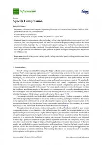
Figure 4: Datasets used for evaluation. From left to right: citadel, city, San Miguel and arena.
Offset compression We observe that the offset from a node to its first child is always +1 (see Fig. 2), implying that this offset can be stored implicitly. Further, offsets are typically small in the lower levels of the tree due to the depth-first assignment. Hence, fewer bits are required to represent the offset. To this extent, we analyze each level and find the minimum number of bits required to encode offsets in this level. We round up to bytes for performance reasons, as a texture lookup on the GPU retrieves at least a single byte. In practice, a two-byte offset is sufficient for the lowest five levels in all our examples, leading to a significant improvement. Four or even five bytes are still required for offsets on the highest levels, but these represent much fewer nodes (≈ 0.1%), which makes the increased memory usage non-critical.
Table 1: Decoupling and palette compression. The numbers are computed for a 64K 3 resolution (16 hierarchical tree levels) using non-quantized, 24-bit colors for the attributes. Scenes Geometry
Citadel
City
San Miguel
Arena
DAG voxels (M)
18.3
10.2
18.8
34.7
DAG size (MB)
382
207
395
737
With offsets (MB)
693
374
719
1342
4760
10487
14788
3263
24-bit colors Λ (M) λ (M)
Pointer compression We apply the same compression technique as for the offsets to the child pointers as well. While this leads to a slight improvement, the compression does not work as well as for offsets, since the levels that contain most pointers generally require the full four bytes per pointer. However, we observe that some subtrees are used significantly more often than others, which makes entropy encoding [BRGIG∗ 14] a well-suited candidate for memory reduction. We create a table of the most common pointers per level – much in the spirit of our material array in Sec. 4.2 – which is sorted by occurrence in descending order. In the DAG, we then store only an index into the pointer table, which is usually smaller than the original pointer and can be represented with fewer bits. In practice, we found the following setup to be most effective: each pointer is initially assumed to be one byte. Its first two bits store the type, which then indicates the pointer’s actual bit length. Two bits can encode four types; the first three are used to indicate if 6, 14, or 22 bits are used to encode a pointer into the lookup table, and the last type is reserved to indicate that the remaining 30 bits correspond to an absolute pointer (as before, this ensure multiples of bytes). The latter could also be increased to 46 bits, but 30-bit pointers proved sufficient for the DAG nodes in all our examples. While we achieve significant compression with the entropy encoding, it does decrease the performance, as evaluated in Sec. 5.
A (MB) e + M (MB) A PC (MB)
Compression rate
1.66
1.42
3.15
1.57
13619
30004
42309
9336
11922
26257
38792
8174
10124
24051
10877
2220
74%
80%
26%
24%
colors, and is a good test case for a realistic dataset. The datasets were produced by voxelizing triangle meshes through depth peeling [Eve01], using the standard extension proposed by Heidelberger et al. [HTG03]. While our compression schemes can handle any spatially coherent data, in practice, we evaluate our method using colors and normals, which are crucial for realistic lighting. We define the compression rate as the memory size of the compressed data over that of the uncompressed data, expressed as a percentage. In the following, we discuss the results of our compression components separately as described in Sec. 4. Starting with the palette approach, we then analyze the gain of lossless and lossy compression, and present the results of our offset and pointer compression. Next, we compare our approach to existing techniques. Finally, we present results to illustrate the performance of our method and discuss its properties before showcasing several application scenarios.
5. Results
5.1. Decoupling and palette compression
Our method aims at large sparse navigable scenes. For evaluation, we deliberately choose a set of very distinct datasets (see Fig. 4): architectural structures (the citadel and city scene); complex geometry (tree and plants in the San Miguel scene); and a 3D model obtained from real-life photographs using floating-scale surface reconstruction [FG14] (arena scene), which is noisy, contains diverse
We show statistics for the DAG-based geometry encoding and the attribute array for our four test scenes in Tab. 1. We list the number of DAG voxels in millions, as well as the memory footprints in MB of the standard and offset-augmented version of the DAG, which is needed to decouple geometry and attributes. The additional offset and pointer compression is analyzed in Sec. 5.3. c 2016 The Author(s)
c 2016 The Eurographics Association and John Wiley & Sons Ltd. Computer Graphics Forum
B. Dado, T. R. Kol, P. Bauszat, J.-M. Thiery & E. Eisemann / Geometry and Attribute Compression for Voxel Scenes
Table 2: Attribute quantization memory footprints and quality. The numbers are computed for a 64K 3 resolution using 24-, 14- and 12bit colors, and for a 32K 3 resolution using 32- and 12-bit ONVs. Scenes 24-bit colors
Citadel
City
San Miguel
Arena
A (MB)
13619
30004
42309
9336
14-bit colors PC (MB)
3645
8163
4495
656
Mean RGB err.
2/1/2
2/1/2
2/2/2
2/1/2
Max. RGB err.
20/4/5
6/7/7
9/26/11
34/5/4
Mean ∆E
1.05
0.91
0.80
0.90
Max. ∆E
2.57
2.44
3.00
2.36
Comp. rate
27%
27%
11%
7.0%
12-bit colors PC (MB)
2609
5703
3099
438
Mean RGB err.
3/2/3
3/2/3
3/2/3
3/2/3
Max. RGB err.
10/7/29
11/12/11
11/9/25
48/5/3
1.72
1.60
1.47
1.75
Mean ∆E Max. ∆E
4.25
3.85
5.28
4.38
Comp. rate
19%
19%
7.3%
4.7%
4496
9994
14081
3110
32-bit ONVs A (MB) PC (MB)
912
417
2678
2151
Comp. rate
20%
4.2%
19%
69%
12-bit ONVs PC (MB)
135
85.9
407
464
Mean/max. err.
2◦ /8◦
2◦ /8◦
2◦ /8◦
2◦ /8◦
Comp. rate
3.0%
0.9%
2.9%
14%
memory gain of our result using palette compression and quantized colors (14 and 12 bits). To assess the fidelity of our quantization, we report the mean absolute error for each RGB channel over all voxels, as well as the maximum deviation. However, since these numbers do not always give a good impression of perceptual quality, we further report mean and maximum ∆E-values as defined by the CIE94 standard. We use kL = 1, K1 = 0.045 and K2 = 0.015 and the D65 illuminant as the reference white, as per graphics industry standards [Kle10]. Finally, we show the compression rates obtained with our palette approach for quantized colors. To illustrate the impact during rendering, Fig. 5 shows images from two viewpoints in the citadel scene. These exhibit many unique values, as well as color and normal gradients, which represent a difficult case for quantization. We provide SSIM values (a perceptual similarity metric, where SSIM = 1 means identical) for every image [WBSS04], comparing the result to its non-quantized counterpart. We note that 14-bit colors produce very good results, and even for 12-bit colors the only indication of quantization is the presence of minor banding artifacts at some locations. For 10-bit colors the quality is reduced, as evidenced by the color difference image, but the result is still relatively close to the reference. Similarly, we report memory footprints for normals in Tab. 2. We consider a 32K 3 resolution with 32-bit ONVs as a reference, since 96-bit normals at 15 levels could not be handled by our hardware, and the mean error for 32-bit ONVs compared to regular 96-bit normals is only 0.001◦ , with a theoretically proven maximum error below 0.004◦ . For quantization, we use 12-bit ONVs, for which we report mean and maximum errors in degrees and show the attained compression rates. As expected, normals compress better than colors for scenes that contain many aligned surfaces, like the city scene. Visually, 16-bit normals produce results indistinguishable from the 32-bit reference while 12-bit and 10-bit normals produce minor and more visible banding on smoothly varying surfaces, respectively (see Fig. 5). Nonetheless, for diffuse shading, such artifacts are barely perceivable and even 10 bits may suffice. For effects like specular reflections, 16-bit normals are preferred. Tab. 1 and 2 show that the memory footprint of the attributes is now potentially compressed to a similar order of magnitude as the geometry. We can see that the combined use of quantization and our palette compression is very fruitful in practice.
Further, Tab. 1 shows the number of attributes Λ, which equals the SVO node count, and the number of unique attributes λ, both in millions. The memory size in MB of the attribute array (indicated as A) exceeds that of the DAG by far. Still, λ is usually much smaller than Λ; indeed, the memory cost of the attribute array can e already be decreased by using a material array (indicated as A+M). Using our palette compression (indicated as PC) reduces the cost again; we report the compression rate by comparing to the original attribute array A. While overall significant, the use of a lossless scheme seems overly conservative in most practical scenarios and implies that even very similar attributes will have to be represented individually. By allowing for a slightly lossy quantization, the attribute costs can be reduced significantly.
Furthermore, combining colors, normals or even reflectance information rarely leads to a linear increase of memory. For example, the night-time version of the city scene at a 32K 3 resolution (Fig. 8, left) uses 12-bit colors, 10-bit normals, and 8-bit reflectance information. The total memory footprint is 1492 MB, compared to 1186 MB for just encoding colors. This means that the normals and reflectance information yield a 25.8% overhead, even though the voxel data grew by 150%. This outcome is a consequence of materials with similar colors often having similar normals and reflectance values as well (e.g., a roughly uniformly colored wall).
5.2. Attribute quantization
5.3. Offset and pointer compression
Data quantization might impact precision, but leads to an often similar appearance and a large memory benefit. In Tab. 2, we show the size of the attribute array for 24-bit colors again, and the drastic
To evaluate our geometry compression, we compare the effect of all our offset and pointer optimizations separately. In Tab. 3, we reiterate the memory footprint of the standard offset-augmented DAG (as
c 2016 The Author(s)
c 2016 The Eurographics Association and John Wiley & Sons Ltd. Computer Graphics Forum
B. Dado, T. R. Kol, P. Bauszat, J.-M. Thiery & E. Eisemann / Geometry and Attribute Compression for Voxel Scenes 12-bit colors
14-bit colors
10-bit colors 10
24-bit colors
SSIM = 0.9908
SSIM = 0.9775
SSIM = 0.9463
16-bit normals
12-bit normals
10-bit normals
SSIM = 0.9963
SSIM = 0.9802
SSIM = 0.9492
Magnitude of color difference
5
32-bit normals
0 Magnitude of color difference
Figure 5: Perceptual quality of our color and normal quantization. We show the quantized result for 14-bit, 12-bit and 10-bit colors, with √ their corresponding magnitude of the color difference (i.e., dR2 + dG2 + dB2 ) per pixel. We do the same for quantized normals, showing the results for 16-bit, 12-bit and 10-bit normals. The difference values are mapped using the color map on the right, where a difference of 10 corresponds to a bright yellow color. We further report SSIM values for each image to assess the perceptual similarity [WBSS04].
Table 3: Offset and pointer compression for a 64K 3 resolution. Scenes DAG size (MB)
Citadel
City
San Miguel
Arena
Uncompressed
693
374
719
1342
Implicit offset
623
335
647
1210
Offset compression
499
271
505
907
Pointer compression
629
330
623
1228
8-bit childmask
641
345
665
1243
Pointer entropy
543
290
531
1027
Combined
348
186
316
591
Compression rate
50%
50%
44%
44%
in Tab. 1). We then report results for implicitly storing the first child offset; the per-level byte-precise offset compression; the per-level byte-precise compression for pointers; 8-bit childmasks (the original DAG uses 24 bits of padding); pointer entropy encoding; and, finally, a combination of all these techniques, for which the shown compression rate compares to the standard offset-augmented DAG. We can see that our approach is quite effective, as we observe that the final memory footprint is on par or even less than the memory cost of the original DAG without the offsets (see Tab. 1).
5.4. Comparison Now that we have discussed all components, we can compare our compression scheme to existing techniques. As we use 12-bit colors for the comparison, the memory footprint of our complete data structure now equals the geometry size for the combined methods in Tab. 3 plus the attribute size for 12-bit colors in Tab. 2. We compare the cost per voxel of our approach to four other techniques; SVOs, PSVOs [SK06], ESVOs [LK10], and CDAGs (naively adding colors to the original DAG [KSA13]). For the standard SVO implementation, the memory footprint is computed as follows: we have an 8-bit childmask, a 32-bit pointer, and a 12-bit color value for every node – note that the leaf nodes have no childmask or pointer. The PSVO contains exactly the same data in every node, except for the child pointer. Besides voxel attributes, ESVOs store additional contour data, but also make use of compression. For color, a DXT1 compression is used while normals are compressed using a novel scheme, which is also lossy, but provides up to 14 bits of precision per axis. In this section, we report ESVO memory footprints as obtained by using the implementation supplied by the authors, which makes use of the aforementioned attribute and contour-based compression. Finally, we have the original DAG [KSA13], augmented with color data, so that every node contains a 32-bit childmask, one to eight 32-bit pointers, and a 12-bit color value (CDAGs). For a direct comparison of our attribute compression to that used c 2016 The Author(s)
c 2016 The Eurographics Association and John Wiley & Sons Ltd. Computer Graphics Forum
B. Dado, T. R. Kol, P. Bauszat, J.-M. Thiery & E. Eisemann / Geometry and Attribute Compression for Voxel Scenes
Bytes per voxel
6
Citadel
5
6
City
5
6
San Miguel
5
6
4
4
4
4
3
3
3
3
2
2
2
2
1
1
1
1
0
0
0
10 11
12 13 14 SVO levels
15 16
10 11
12 13 14 SVO levels
15 16
10 11
12 13 14 SVO levels
15 16
Arena
5
0
10 11
12 13 14 SVO levels
SVO PSVO ESVO CDAG Ours
15 16
Figure 6: Memory usage per voxel for our test scenes at different SVO levels. We compare our approach to a colored SVO, PSVOs [SK06], ESVOs [LK11] and a naive colored DAG implementation (CDAGs). Note that the ESVO implementation was unable to load the arena scene.
Table 4: Comparison to the state of the art for a 64K 3 resolution. Scenes Citadel
City
San Miguel
Arena
SVO voxels (M)
4760
10487
14788
3263
Size (MB)
13285
27966
39122
9520
Bytes/voxel
2.93
2.80
2.77
3.06
PSVO size (MB)
8105
17595
24748
5638
Bytes/voxel
1.79
1.76
1.75
1.81
ESVO voxels (M)
1533
2782
1168
Size (MB)
10374
18506
8174
Bytes/voxel
2.29
1.85
0.58
CDAG voxels (M)
286
629
251
117
Size (MB)
5540
11922
4791
2326
Bytes/voxel
1.22
1.19
0.34
0.75
18
10
19
34
Our voxels (M) Geometry (MB)
348
186
316
591
Attributes (MB)
2609
5703
3099
438
Total size (MB)
2957
5889
3415
1029
Bytes/voxel
0.65
0.59
0.24
0.33
Compression rate
22%
21%
8.7%
11%
by ESVOs, we built the Sibenik scene at a 8K 3 resolution. Here, ESVOs reported a memory footprint of 2120 MB without using contours [LK10]. Not using contours is important, as, contrary to geometry, a similar quality as regular colored SVOs can only be achieved for attributes if they are not cut off during traversal. Further, as the data quality for ESVOs is not evaluated, it is difficult to provide a comparison; hence, we use 24-bit colors and 32-bit ONV normals for the palette compression, which ensures better quality than the lossy schemes applied by ESVOs. Our palette compression is more flexible when compared to the constant DXT1 rate, which results in only 1171 MB for our entire data structure. Fig. 6 and Tab. 4 illustrate that our approach outperforms other methods by a significant margin. We report bytes per voxel for all techniques, always with reference to the SVO node count. We list c 2016 The Author(s)
c 2016 The Eurographics Association and John Wiley & Sons Ltd. Computer Graphics Forum
Table 5: Construction times in minutes at different resolutions for our four test scenes, using the naive colored DAG implementation and our decoupling and palette compression, with 12-bit colors. Scenes Resolution
Citadel
City
San Miguel
Arena
3
1.60/2.58
0.75/6.01
1.40/5.31
1.08/1.83
8K 3
2.65/17.1
2.93/30.3
5.90/22.0
3.13/7.35
10.8/64.5
13.2/217
20.0/157
10.0/21.3
4K
16K
3
Frame number
Figure 7: Rendering times while navigating through the citadel scene at a 32K 3 resolution, obtained by raycasting in full HD.
the actual voxel count in millions for SVOs, ESVOs, CDAGs, and our method separately. We show the geometry and attribute size separately and combined for our method. Finally, we report compression rates as compared to a standard SVO implementation. 5.5. Performance Construction As our focus was mostly on compression quality, not performance, we did not investigate significant acceleration techniques for the DAG algorithm, nor for our palette compression. Still, the construction times for building our data structure are interesting, as they illustrate the computational overhead of involving attributes. In Tab. 5, we report timings on an i5 CPU in minutes for both standard colored DAGs (before the slash) and our method
B. Dado, T. R. Kol, P. Bauszat, J.-M. Thiery & E. Eisemann / Geometry and Attribute Compression for Voxel Scenes
Figure 8: Several applications of our compressed SVO. From left to right: encoding reflectance information in materials for the city scene, rendered at a resolution of 32K 3 ; color bleeding in the CrySponza scene, at an SVO resolution of 4K 3 , using 16 samples per pixel, and secondary and tertiary ray tracing at a 5123 resolution; rendering of a dense dataset of a Christmas tree at a 512 × 512 × 999 resolution.
(after the slash); for the latter, we see an increase up to an order of magnitude. Still, it is feasible to compute high-resolution scenes on commodity hardware, and the slow construction does not hurt performance during rendering. The construction time depends mostly on the number of compression attempts that our algorithm explores; if large blocks are already found in the first phase, as for the arena scene, the cost of the palette compression is significantly reduced. Rendering We did not particularly optimize our rendering algorithm; in each frame, we cast rays from the camera and traverse the SVO with a standard stack-based approach to find the first intersecting voxel that projects to an area smaller than a pixel. To still demonstrate that our method is capable of real-time performance, Fig. 7 shows timings for a walk-through in the citadel scene in full HD at a 32K 3 resolution, obtained using an NVIDIA Titan X. We compare the rendering times for palette compression, per-level byte-precise offsets, and using all our compression techniques, to naive colored DAGs (CDAGs). We can conclude that palettes and offset compression have some impact on the performance, but still enable real-time rendering while yielding significant compression rates. The entropy encoding on the other hand has a bigger influence and we only achieve interactive rates. Still, it can be useful for memory gain, especially when the geometry is relatively large, like for the arena scene (see Tab. 4). Further, the rendering cost is several orders of magnitude lower than for pointerless solutions while still avoiding high memory costs. 5.6. Applications To demonstrate the versatility of our approach, and of SVOs in general, we showcase several applications. Like the original DAG, we are able to obtain high-resolution hard shadows for the whole scene. With normals, however, we can look into more interesting applications, such as reflections, by shooting secondary rays while maintaining real-time performance (Fig. 8, left). We have also implemented a simple approach to color bleeding through single-bounce global illumination (Fig. 8, middle). We shoot multiple secondary rays via stratified sampling of the hemisphere – which means the samples are uniformly distributed, but contain a random offset – and then shoot tertiary rays from the
intersecting voxels to determine if they are in shadow. We attain interactive rates with 8 secondary rays per pixel. Since our method, like the DAG, exploits both similarity and sparsity, we can to some extent compress dense data as well (Fig. 8, right). For the shown Christmas tree, we are able to obtain a lossless compression rate of 38.6% when comparing our complete data structure to the original input file, which is approaching state-ofthe-art methods for dense datasets (29.4%) [GWGS02]. When applying a simple filtering to remove scanning noise in the air, we additionally profit from the sparsity and achieve rates below 10%. 6. Conclusions We have presented a novel SVO compression scheme, which relies on the decoupling of geometry from additional voxel data. Our mapping is efficient and introduces little overhead, enabling separate compression methods for topology and voxel attributes. Furthermore, we introduced compression schemes for child pointers, which also reduces the cost of traditional DAGs. For attribute compression, we proposed a combination of our quantization and our lossless palette approach, which implicitly exploits spatial coherence. We showed that our solution reduces memory usage from 4.49 times (for the citadel) up to 11.5 times (for San Miguel) compared to standard SVO implementations. Our method outperforms state-of-the-art SVO compression methods for all test scenes. The high compression rates allow us to store colored SVOs with up to 17 levels (a voxel resolution of 128K 3 ) completely on the GPU. We demonstrated real-time rendering performance using commodity hardware and showcased several applications such as color bleeding and reflections, for which additionally normal and reflectance attributes were encoded. For future work, investigating more advanced material properties for the voxel data (e.g., BRDFs encoded via spherical harmonics or transparency values) are interesting directions. Acknowledgements This work was partially supported by the FP7 European Project Harvest4D and the Intel VCI. c 2016 The Author(s)
c 2016 The Eurographics Association and John Wiley & Sons Ltd. Computer Graphics Forum
B. Dado, T. R. Kol, P. Bauszat, J.-M. Thiery & E. Eisemann / Geometry and Attribute Compression for Voxel Scenes
References [BRGIG∗ 14]
BALSA RODRÍGUEZ M., G OBBETTI E., I GLESIAS G UI J., M AKHINYA M., M ARTON F., PAJAROLA R., S UTER S.: Stateof-the-art in compressed GPU-based direct volume rendering. Computer Graphics Forum 33, 6 (2014), 77–100. 1, 2, 6 TIÁN
[CDE∗ 14] C IGOLLE Z. H., D ONOW S., E VANGELAKOS D., M ARA M., M C G UIRE M., M EYER Q.: A survey of efficient representations for independent unit vectors. Journal of Computer Graphics Techniques 3, 2 (2014), 1–30. 2, 5 [CNLE09] C RASSIN C., N EYRET F., L EFEBVRE S., E ISEMANN E.: GigaVoxels: Ray-guided streaming for efficient and detailed voxel rendering. In Proc. of I3D (2009), pp. 15–22. 2 [CNSE10] C RASSIN C., N EYRET F., S AINZ M., E ISEMANN E.: GPU Pro. AK Peters, 2010, ch. X.3 Efficient rendering of highly detailed volumetric scenes with GigaVoxels, pp. 643–676. 2 [Eve01] E VERITT C.: Interactive order-independent transparency. Tech. rep., NVIDIA Corporation, 2001. 6 [FG14] F UHRMANN S., G OESELE M.: Floating scale surface reconstruction. Trans. on Graphics 33, 4 (2014), 46. 6 [GMIG08] G OBBETTI E., M ARTON F., I GLESIAS G UITIÁN J. A.: A single-pass GPU ray casting framework for interactive out-of-core rendering of massive volumetric datasets. The Visual Computer 24, 7 (2008), 797–806. 2 [GWGS02] G UTHE S., WAND M., G ONSER J., S TRASSER W.: Interactive rendering of large volume data sets. In Proc. of VIS (2002), pp. 53– 60. 2, 10 [HTG03] H EIDELBERGER B., T ESCHNER M., G ROSS M. H.: Real-time volumetric intersections of deforming objects. In Proc. of VMV (2003), pp. 461–468. 6 [JMG16] JASPE V ILLANUEVA A., M ARTON F., G OBBETTI E.: SSVDAGs: Symmetry-aware sparse voxel DAGs. In Proc. of I3D (2016). 2 [JT80] JACKINS C. L., TANIMOTO S. L.: Oct-trees and their use in representing three-dimensional objects. Computer Graphics and Image Processing 14, 3 (1980), 249–270. 1, 2 [Kle10]
K LEIN G. A.: Industrial color physics. Springer, 2010. 7
[KSA13] K ÄMPE V., S INTORN E., A SSARSSON U.: High resolution sparse voxel DAGs. Trans. on Graphics 32, 4 (2013), 101. 2, 3, 8 [KSA15] K ÄMPE V., S INTORN E., A SSARSSON U.: Fast, memoryefficient construction of voxelized shadows. In Proc. of I3D (2015), pp. 25–30. 2 [LH06] L EFEBVRE S., H OPPE H.: Perfect spatial hashing. Trans. on Graphics 25, 3 (2006), 579–588. 2 [LH07] L EFEBVRE S., H OPPE H.: Compressed random-access trees for spatially coherent data. In Proc. of EGSR (2007), pp. 339–349. 2 [LK10] L AINE S., K ARRAS T.: Efficient sparse voxel octrees – analysis, extensions, and implementation. Tech. rep., NVIDIA Corporation, 2010. 1, 8, 9 [LK11] L AINE S., K ARRAS T.: Efficient sparse voxel octrees. Trans. on Visualization and Computer Graphics 17, 8 (2011), 1048–1059. 2, 9 [Mea82] M EAGHER D.: Geometric modeling using octree encoding. Computer Graphics and Image Processing 19, 2 (1982), 129–147. 1, 2 [MSS∗ 10] M EYER Q., S ÜSSMUTH J., S USSNER G., S TAMMINGER M., G REINER G.: On floating-point normal vectors. Computer Graphics Forum 29, 4 (2010), 1405–1409. 2, 5 [NLP∗ 12] N YSTAD J., L ASSEN A., P OMIANOWSKI A., E LLIS S., O L SON T.: Adaptive scalable texture compression. In Proc. of HPG (2012), pp. 105–114. 2 [SAM05] S TRÖM J., A KENINE -M ÖLLER T.: iPACKMAN: Highquality, low-complexity texture compression for mobile phones. In Proc. of HWWS (2005), pp. 63–70. 2 c 2016 The Author(s)
c 2016 The Eurographics Association and John Wiley & Sons Ltd. Computer Graphics Forum
[SK06] S CHNABEL R., K LEIN R.: Octree-based point-cloud compression. In Proc. of SPBG (2006), pp. 111–120. 2, 8, 9 [SKOA14] S INTORN E., K ÄMPE V., O LSSON O., A SSARSSON U.: Compact precomputed voxelized shadows. Trans. on Graphics 33, 4 (2014), 150. 2 [WBSS04] WANG Z., B OVIK A. C., S HEIKH H. R., S IMONCELLI E. P.: Image quality assessment: From error visibility to structural similarity. IEEE Trans. on Image Processing 13, 4 (2004), 600–612. 7, 8 [Wil15] W ILLIAMS B. R.: Moxel DAGs: Connecting material information to high resolution sparse voxel DAGs. Master’s thesis, California Polytechnic State University, 2015. 2 [Xia97] X IANG Z.: Color image quantization by minimizing the maximum intercluster distance. Trans. on Graphics 16, 3 (1997), 260–276. 2, 5