Aug 4, 2016 - mogeneous solution of a spatially extended multispecies model, .... Laplacian on a continuous support. .... on a symmetric network support.
Global topological control for synchronized dynamics on networks. Giulia Cencetti,1, 2 Franco Bagnoli,3, 2 Giorgio Battistelli,1 Luigi Chisci,1 Francesca Di Patti,3, 2 and Duccio Fanelli3, 2
arXiv:1608.01572v1 [cond-mat.stat-mech] 4 Aug 2016
1
Dipartimento di Ingegneria dell’Informazione, Universit` a di Firenze, Via S. Marta 3, 50139 Florence, Italy 2 INFN Sezione di Firenze, via G. Sansone 1, 50019 Sesto Fiorentino, Italia 3 Universit` a degli Studi di Firenze, Dipartimento di Fisica e Astronomia and CSDC, via G. Sansone 1, 50019 Sesto Fiorentino, Italia A general scheme is proposed and tested to control the symmetry breaking instability of a homogeneous solution of a spatially extended multispecies model, defined on a network. The inherent discreteness of the space makes it possible to act on the topology of the inter-nodes contacts to achieve the desired degree of stabilization, without altering the dynamical parameters of the model. Both symmetric and asymmetric couplings are considered. In this latter setting the web of contacts is assumed to be balanced, for the homogeneous equilibrium to exist. The performance of the proposed method are assessed, assuming the Complex Ginzburg-Landau equation as a reference model. In this case, the implemented control allows one to stabilize the synchronous limit cycle, hence time-dependent, uniform solution. A system of coupled real Ginzburg-Landau equations is also investigated to obtain the topological stabilization of a homogeneous and constant fixed point. PACS numbers: 89.75.-k 89.75.Kd 89.75.Fb 02.30.Yy 05.45.Xt
INTRODUCTION
Self-organized collective dynamics may emerge in systems constituted by many-body interacting entities [1, 2]. This is a widespread observation in nature which fertilized in a cross-disciplinary perspective to ideally embrace distinct realms of investigations. Convection instabilities in fluid dynamics, weak turbulences and defects are among the examples that testify on the inherent ability of physical systems to yield coherent dynamical behaviors [3]. Insect swarms and fish schools exemplify the degree of spontaneous coordination that can be reached in ecological applications [4], while rhythms production and the brain functions refer to archetypical illustrations drawn from biology and life science in general [5–10]. The mathematics that underlies patterns formation focuses on the dynamical interplay between reaction and diffusion processes. Usually, reaction-diffusion models are defined on a regular lattice, either continuous or discrete [11]. In many cases of interest, it is however more natural to schematize the system as a network, bearing a heterogeneous and complex structure [7, 12–15]. To account for the hierarchical organization in multiple nested layers, networks of networks can be also considered [16– 24]. Imagine microscopic fluctuations to shake a stationary stable, homogeneous equilibrium of the analyed, spatially extended, system. Under specific conditions, the imposed fluctuations get self-consistently enhanced by an intrinsic resonance mechanism, which is ultimately triggered by the spatial component of the dynamics: instabilities seeded by random perturbations are often patterns precursors and eventually materialize in beautiful patchy motifs for the concentration of the mutually interacting species [6, 25–34]. These are the byproduct of the celebrated Turing instability, named after Alan Turing who first conceived the symmetry breaking mechanism from
which the process originates [35]. For reaction-diffusion systems hosted on a graph, the instability typifies a characteristic asymptotic segregation in rich (resp. poor) nodes of activators (resp. inhibitors), a non homogeneous attractor that unavoidably emanates from the initially synchronous configuration [7, 36, 37]. In many cases of interest it is however important to oppose the natural drive to pattern formation, by preserving (or recovering) the synchronized state [38, 39]. Synchronization plays indeed a pivotal role in many branches of science: the efficient coordination of a multitude of events is often decisive to have a system operated as a unison orchestra. In an alternating current electric power grid, one needs to match the speed and frequency of any given generator to the other sources of the shared network [40–42]. In neuroscience, patterns of synchronous firings are promoted by dedicated neuronal feedbacks. Circadian rhythms are another example that certifies the ubiquitous tendency towards entrainable oscillations as displayed by a vast plethora of biological processes [5, 43]. In computer science, synchronization is customarily referred to as consensus [44], a form of final agreement, stationary or time dependent, which is reached by a crowd of interacting agents. Given these premises it is in general important to devise apt control strategies that enable one to stabilize, and possibly preserve, the synchronous regime. The control is classically applied to the reactive component of the dynamics, and ultimately shape the local interaction between constitutive elements [45]. Global, mean field term can be also accommodated for so as to induce the sought behavior. When the dynamics flow on a network, topology matters and does play a prominent role in eliciting the instability [14, 36]. This observation motivates in the search of alternative control protocols, which leave the reaction part unchanged, while acting on the under-
2 lying web of inter-nodes connections [46, 47]. The aim of this paper is to contribute along this direction, by proposing a viable topological approach which is fully rooted on first principles.
To illustrate the proposed method we shall first operate in the framework of the Complex Ginzburg-Landau Equation (CGLE) [48] a prototypical model for nonlinear physics, whose applications range from superconductivity, superfluidity and Bose-Einstein condensation to liquid crystals and strings in field theory. The CGLE assumes a population of oscillators, described in terms of their complex amplitude and mutually coupled via a diffusive-like interaction. This is mathematically described in terms of a discrete Laplacian operator. The CGLE admits a uniform fully synchronized solution, the spatially extended replica of the periodic orbit displayed by the system in its a-spatial version, provided the Laplacian is balanced (equal incoming and outgoing connectivity) [49]. Hereafter, we shall assume that the nodes of the network where oscillators lie are initially paired (and the reaction parameters set) so as to make the system unstable to externally injected, non homogeneous, perturbations. The network of connections is then globally reshaped (keeping the reaction parameters unchanged) to regain the stability of the synchronized, time dependent, solution. We will then move forward to considering a system of coupled (real) Ginzburg-Landau equations [50], which admits a stationary stable fixed point. Turing-like instabilities will be controlled, hence formally impeded, with a supervised intervention targeted to the net of interlaced couplings.
The paper is organized as follows. In the next section we will introduce the CGLE and carry out a linear stability analysis to delineate the conditions that make the spatially extended, homogenous limit cycle solution stable. We will in particular elaborate on the remarkable differences that arise when the system involves a finite and discrete collection of interlinked oscillators, as opposed to the reference case where the population of elementary constituents is made infinite and continuous. In Section III we will provide the mathematical basis for the proposed control method. The approach will be successfully tested by operating with the CGLE and assuming a symmetric network. In Section IV, we will consider a directed, although balanced, network of couplings and extend to this setting the analysis. Finally in Section V we will sum up and draw our conclusions. The appendix is devoted to discussing the stabilization of a constant homogeneous fixed point, and proving, also in this respect, the adequacy of the proposed recipe.
COMPLEX GINZBURG-LANDAU EQUATION: LINEAR STABILITY ANALYSIS
Consider an ensemble made of N nonlinear oscillators and label with Wi their associated complex amplitude, where i = 1, ..., N . Each individual oscillator obeys to a CGLE which, as will be clarified in the following, combines linear and nonlinear (cubic) contributions. In addition, we assume the oscillators to be mutually coupled via a diffusive-like interaction which is mathematically exemplified via the discrete Laplacian operator. To fix ideas consider as an example the simplified setting in which the oscillators are coupled to nearest neighbors only, on a one dimensional lattice complemented with periodic boundary conditions. The network of connections yields a binary adjacency matrix, termed A: the entry Aij is set to one if nodes i and j are paired together, or zero if the link is absent. The associated discrete Laplacian operator ∆ results in a circulant matrix with three non trivial entries per row, namely ∆ii = −2, ∆i,i+1 = 1 and ∆i,i−1 = 1. In general, a complex web of inter-nodes connections yields a heterogenous network, potentially directed (Aij 6= Aji ) P and weighted. In thisP case, let us in denote with kiout = A (resp. k = ji i j j Aij ) the outgoing (resp. ingoing) connectivity of generic node i. In our study we will deal with symmetric or balanced and directed networks, hence kiout = kiin ≡ ki . The elements of the Laplacian matrix ∆ are therefore defined as ∆ij = Aij − ki δij , where δij stands for the usual Kronecker δ. The spatially extended CGLE can be hence cast in the form: X d Wj = Wj − (1 + ic2 )|Wj |2 Wj + (1 + ic1 )K ∆jk Wk dt k (1) where c1 and c2 are real parameters, which can be externally assigned. The index j runs from 1 to N , the size of the inspected system. Here, K is a suitable parameter setting the coupling strength. We shall begin by considering a symmetric adjacency matrix and postpone to a later stage the case of a directed, though balanced, network of couplings. For pedagogical reasons, let us start by considering a regular lattice, embedded on a Euclidean space of arbitrary dimension. By performing the continuum limit, i.e assuming the linear distance between neighbor nodes to asymptotically vanish, one can formally replace the discrete variable Wj (t) (j = 1, 2, · · · , N ) with its continuous counterpart W (r, t). Here, W (r, t) ∈ C and r identifies the space location. Under these conditions, the discrete operator ∆ transforms into ∇2 , the standard Laplacian on a continuous support. For this reason, and with a slight abuse of language, we shall often employ the adjective spatial to tipify the nature of the coupling, even when the network of oscillators is not necessarily
3 bound to a physical space. As a preliminary remark we note that W LC (t) = e−ic2 t is a homogenous solution of the CGLE, both in its discrete or continuous, spatially extended, versions. This latter can be referred to as the limit cycle (LC) solution, since it results from a uniform, fully synchronized, replica of the periodic orbit displayed by the system in its a-spatial (K = 0) version. In the remaining part of this section, we shall determine the stability of the LC solution. We will deal at first with the continuous version of the model and re-derive for completeness the conditions for the onset of the so called Benjamin-Feir instability [51, 52]. The peculiarities that stem from assuming a discrete and heterogeneous web of symmetric couplings will be also reviewed. To assess the stability of the LC solution we introduce a non homogeneous perturbation, both in phase and amplitude: W (r, t) = W LC (t)[1 + ρ(r, t)]eiθ(r,t) .
(2)
Linearizing around the LC (ρ(r, t) = 0, θ(r, t) = 0) one readily obtains: � � � �� � � � � � d ρ −2 0 ρ 1 −c1 2 ρ = +K ∇ . (3) −2c2 0 θ c1 1 θ dt θ To solve the above linear problem we perform a spacetime Fourier transform: RR ρ(r, t) = R R dωdkeiωt eik·r ρk θ(r, t) = dωdkeiωt eik·r θk .
real part of λ (the dispersion relation λRe ) is positive. Notice that λ(0) = λRe (0) = 0, as expected, based on a obvious argument of internal coherence. Expanding Eq. (6) for small k returns λRe ' −(1 + c1 c2 )k 2 . The stability of the synchronized LC solution is therefore lost when (1 + c1 c2 ) < 0, the standard condition for the onset of the Benjamin-Feir instability. We now turn to considering the case of a heterogenous, although symmetric, network of connections among oscillators. To investigate the conditions that are to be met for a symmetry breaking instability of the homogeneous LC solution to develop, we proceed in analogy with the above and set Wj (t) = W LC (t)[1 + ρj (t)]eiθj (t) , with a clear meaning of the symbols. Plugging this latter expression in the CGLE (1) and expanding to the first order in the perturbation amount, one obtains the obvious generalization of system (3): d dt
�
ρj θj
�
�
�� � � � � � −2 0 ρj 1 −c1 X ρk = + ∆jk . −2c2 0 θj c1 1 θk k
(7) where we recall that K = 1. For regular lattices, the Fourier transform is usually invoked to solve the system of equations homologous to (7). This amounts to expanding the spatial perturbations on a set of planar waves, the eigenfunctions of the continuous Laplacian operator. When the system is instead defined on a network, an analogous procedure can be employed. To this end, we define the eigenvalues and eigenvectors of the discrete Laplacian operator:
(4) X
A straightforward calculation returns the following condition that should be matched as a necessary consistent requirement for the linear problem to admit a meaningful solution: λ + 2 + Kk 2 det 2c2 + Kc1 k 2
−Kc1 k 2 λ + Kk
2
=0
(5)
with λ = iω and k = |k|. The quantity λ hence assesses the linear growth rate associated to the k-th mode. Without losing generality we will hereafter set the coupling constant to unit (K = 1) and proceed with the calculation to determine the root of the characteristic polynomial with largest real part:
(α)
∆ij φj
(6)
The perturbation that shakes the homogenous and time dependent solution W LC (t) gets exponentially magnified in the linear regime of the evolution provided the
α = 1, ..., N
(8)
j
When the network is undirected, the Laplacian operator is symmetric. Therefore, the eigenvalues Λ(α) are real and the eigenvectors φ(α) form an orthonormal basis. This condition needs to be relaxed when dealing with the more general setting of a directed graph, as we shall discuss in the second part of the paper[57]. The symmetric Laplacian matrix ∆ has a single zero eigenvalue Λ(α=1) corresponding to the uniform eigenvector and all other eigenvalues are negative. The indices α are sorted so as to satisfy 0 = Λ(1) > Λ(2) ≥ · · · ≥ Λ(N ) . The inhomogeneous perturbations ρj and θj can be expanded as:
� q λ(k 2 ) = −k 2 − 1 + −c21 k 4 − 2c1 c2 k 2 + 1.
(α)
= Λ(α) φi
ρj θj
� =
N � (α) � X ρ α=1
θ(α)
(α)
eλt φj .
(9)
By inserting Eq. (9) in Eq. (7) and making use of relation (8) one eventually gets a condition formally equivalent to expression (5). As an important difference, the
4
In Fig. 1 the dispersion relation λRe is plotted versus (α) −ΛRe , for a specific choice of c1 and c2 , so that 1 + c1 c2 < 0. The solid line refers to the continuum setting (α) (−ΛRe → k 2 ,), while circles are obtained when operating with the CGLE, hosted on a Watts-Strogatz network [53]. As anticipated, the discrete collection of points which defines the dispersion relation when a symmetric, finite and heterogenous network of coupling is accommodated for, follows the same profile which applies to the limiting continuum setting. In Fig. 2 the temporal evolution of the system is displayed for a choice of the parameters which corresponds to the unstable dispersion relation of Fig. 1. After a given time the synchronized LC solution is perturbed by insertion of an external source of non homogenous disturbance. This latter grows, as predicted by the linear stability analysis, and yields the irregular patterns displayed for both WRe and |W|2 . Back to Fig. 1, it is however important to realize that the instability actually takes place only when at least one (α) eigenvalue −ΛRe exists in the range where λRe is positive. If the ensemble of discrete modes, which ultimately reflects the topology of the imposed couplings, populates the portion of the dispersion relation with λRe < 0, no instability can develop, even if 1 + c1 c2 < 0. Stated differently the spectral gap ∆(Λ), the difference between the moduli of the two largest eigenvalues of the Laplacian operator (∆(Λ) = |Λ(2) | − |Λ(1) | = |Λ(2) |) should be larger than −2(c1 c2 + 1)/(1 + c21 ), the non trivial root of Eq. (6), for the instability to take place. This observation has been exploited by Nakao in Ref. [49] to propose a novel control strategy aimed at suppressing the Benjamin-Feir instability and thus preserving the initial synchronized regime for a CGLE defined on a symmetric network support. Imagine to start with an unstable condition, which in turn implies to operate with a suitable choice for both the reaction parameters and the network specificity. The key idea of Ref. [49] is to randomly rewire the network so as to make the second eigenvalue progressively more negative. Random moves are accepted or rejected following a Metropolis scheme. The numerical procedure converges to a (globally) modified network which has no eigenvalue in the range where
0 -2
6Re
eigenvalues of the continuous Laplacian, −k 2 , are replaced by the discrete (real and negative) quantities Λ(α) , the eigenvalues of the discrete Laplacian. Insisting on the analogy, it is of immediate evidence that the instability rises for a CGLE defined on a symmetric network when 1 + c1 c2 < 0, a dynamical condition identical to that obtained when operating under the continuous, by definition regular, viewpoint. The quantity Λ(α) constitutes the analogue of the wavelength for a spatial pattern in a system defined on a continuous regular lattice. It is this latter quantity which determines the spatial characteristic of the emerging patterns, when the system is defined on a heterogeneous complex support.
-4 -6 -8 0
1
2
3
4
5
6
7
-$(,) Re FIG. 1: Continuous (solid line) and discrete (blue circles) dispersion relation. Here, c1 = −1.8, c2 = 1.6, K = 1. The network, composed of 100 nodes, is generated from the WattsStrogatz method with rewiring probability 0.8.
λRe > 0. The control is topological since it only affects the couplings that links the oscillators, without acting on the dynamical parameters c1 and c2 . In practice, the discrete network-like system can be made stable for a choice of the parameter that would drive a Benjamin-Feir instability in the continuum limit. Building on these intriguing observations, we will here devise an analytical approach that enables us to implement a similar control protocol, without resorting to an iterative, numerically supervised, rewiring. Importantly, the method that we shall introduce here can be successfully extended to the general case where a directed network of connections is assumed to hold. The next section is devoted to discussing the proposed method.
GLOBAL TOPOLOGICAL CONTROL
As outlined in the preceding section, here we aim at developing an apposite control strategy which acts on the global network of connections, leaving unchanged the dynamical parameters of the model. The method that we shall hereafter discuss takes inspiration from the seminal work of Nakao [49]. There it was shown that a numerically supervised rewiring of the inter-oscillators couplings can stabilize the CGLE, thus preserving the consensus state. Building on similar grounds, we will provide in the following an analytical procedure to achieve the sought stabilization. The proposed method allows one to immediately generate the controlled matrix of contacts, without involving any iterative scheme, thus freeing from
5
1
Node number
20 0.5
40 0
60 -0.5
80 -1
100 10
20
30
40
50
60
Time 1.4 1.2
Node number
20
1
40
0.8 0.6
60
0.4
80 0.2
100 10
20
30
40
50
60
Time FIG. 2: Evolution of WRe (upper panel) and |W|2 (lower panel) versus time, assuming a uniform LC initial condition. At time τ1 = 15, a non homogeneous perturbation is inserted and the synchronized state is consequently disrupted. Here, c1 = −1.8, c2 = 1.6. The nonlinear oscillators are mutually linked via the Watts-Strogatz network, used in depicting the discrete dispersion relation of Fig. 1.
concerns on the numerical convergence. Starting from a condition of instability, as displayed in Fig. 1, we wish to modify the spectrum of the Laplacian operator so as to force the finite and discrete collection of modes to populate the negative branch of the dispersion relation λRe . As emphasized in the previous section, when the network is undirected the discrete dispersion relation superposes to the continuum one (the solid line in Fig. 1). The instability localizes on a finite set of modes, those falling on the positive bump of the curve λRe (k 2 ). Is it possible to alter the network topology so as to make the (neg-
atively defined and real) eigenvalues larger in absolute value than −2(c1 c2 + 1)/(1 + c21 ), the point where the parabola λRe (k 2 ) crosses the horizontal axis, so turning negative? In a figurative sense, we want to slide the discrete points of Fig. 1 onto the curve, as beads on a cord, causing them to reach its negative branch. To answer this question we make use of simple linear algebra tools. Let us start by defining the N × N matrix Φ whose columns are the eigenvectors φ(1) , · · · , φ(N ) of the Laplacian operator ∆. Hence D = Φ−1 ∆Φ, where D is the diagonal matrix formed by the eigenvalues Λ(1) , ..., Λ(N ) . We then calculate the minimal corrections δΛ(α) (α = 1, · · · , N ) that need to be imposed to shift the eigenvalues Λ(α) on the stable side of the dispersion relation. The computed corrections are then organized in a diag0 onal matrix D0 , so that Dαα = δΛ(α) , for α = 1, · · · , N . As a matter of facts, and to keep the formulation general, δΛ(α) ∈ C. For the case of a symmetric network that we are bound to explore within this Section, the quantities δΛ(α) are however real and negative. When the original Λ(α) falls in the region of stability, the corresponding correction δΛ(α) is set to zero. The next step of the procedure is to perform the following transformation ∆0 = ΦD0 Φ−1 and define the controlled matrix ∆c = ∆ + ∆0 . By construction the eigenvalues of ∆c (with the only exception of the zero eigenvalue, α = 1) are smaller than 2(c1 c2 + 1)/(1 + c21 ). Assume for a moment that ∆c can be interpreted as a Laplacian operator. Hence, the obvious conclusion is that we have generated a modified adjacency matrix Ac , hidden inside ∆c , which should engender a negative dispersion relation (when employed in the CGLE, at fixed c1 and c2 ), thus preserving the stability of the synchronized configuration. Before concluding in this respect, one needs to prove that ∆c is indeed a Laplacian matrix, namely that (i) the entries of the matrix are real and P that (ii) every column of the matrix sums up to zero, i (∆c )ij = 0 ∀j). In the following we set down to prove the above properties (for both the symmetric and asymmetric settings), before turning to provide a numerical validation of the devised control procedure. As an important complement, we will also show that symmetry and balancedness are perpetuated from ∆ to ∆c . The elements of ∆c are real. The generic entries of ∆0 can be written as: X 0 ∆0il = Φij Djj (Φ−1 )jl . (10) j
In the symmetric case, the eigenvalues and their corresponding corrections are real. Also the eigenvectors have real entries (vectors in RN ). Hence, the elements of D0 , Φ, Φ−1 are real and, consequently, ∆0ij ∈ R. The undirected case is more complicated to handle. Let us bring into evidence the real and imaginary parts of every ele-
6 ment of Eq. (10). It is immediate to see that the imaginary part of ∆0il reads: (∆0Im )il = X −1 0 = (DIm )jj [(ΦRe )ij (Φ−1 Re )jl − (ΦIm )ij (ΦIm )jl ]+ j
X −1 0 + (DRe )jj [(ΦRe )ij (Φ−1 Im )jl + (ΦIm )ij (ΦRe )jl ]. j
(φ−1 )(k) is the left eigenvector of matrix ∆, relative to the real eigenvalue Λ(k) . Reasoning as above, one can take (φ−1 )(k) to be real and thus (Φ−1 Im )kl = 0. Then, summing up, (∆0Im )il = 0 ∀i, l. Each column of ∆c sums up to zero. Consider X X 0 ∆0il = Φij Djj (Φ−1 )jl = i
(11) To match condition (∆0Im )il = 0, both terms on the right hand side of Eq. (11) should be zero. To prove this fact let us begin by recalling that the eigenvalues of a real asymmetric matrix either are real or are complex and come in conjugate pairs. Consider first the latter case and label with α and β the generic pair of conjugate eigenvalues. By definition ∆φ(α) = Λ(α) φ(α) . Taking the complex conjugate yields ∆(φ(α) )∗ = (Λ(α) )∗ (φ(α) )∗ where (·)∗ stands for the complex conjugate and where use has been made of the condition ∆ = ∆∗ . Recalling that (Λ(α) )∗ = Λ(β) we can immediately conclude that (φ(α) )∗ is an eigenvector of ∆ relative to the eigenvalue Λ(β) and thus φ(β) = (φ(α) )∗ . Hence
ij
X X 0 = (Φ−1 )jl Djj Φij . j
(12)
for every i and (α, β). Consider now the equation (φ−1 )(α) ∆ = Λ(α) (φ−1 )(α)
(13)
with (φ−1 )(α) α-th row of Φ−1 . Proceeding in analogy with the above, one eventually gets: −1 (Φ−1 Re )αl = (ΦRe )βl −1 (ΦIm )αl = −(Φ−1 Im )βl .
(14)
Let us go back to Eq. (11). Performing the summation on j = α and j = β, using Eq. (12) and Eq. (14) and 0 0 the fact that the corrections Dαα and Dββ are complex (α) conjugated as the original eigenvalues Λ and Λ(β) are, we finally conclude that the terms of the sums in Eq. (11) cancel in pairs. Consider now the case of a real eigenvalue Λ(k) . Hence, 0 by definition, (DIm )kk = 0, since, in this case, the stabilization can be solely achieved by acting on the real part of the eigenvalue (see next Section). To prove that (∆Im )il = 0 we need therefore to focus on the second term of Eq. (11), with j = k. Without losing generality (k) (up to a constant scaling factor) φIm = 0: the eigen(k) vector associated to Λ is hence real. The ik entries of matrix Φ are indeed the elements of φ(k) and, for this reason, (ΦIm )ik = 0 ∀i. To conclude the reasoning and eventually prove that (∆0Im )il = 0, one needs to show that (ΦRe )ik (Φ−1 Im )kl = 0. This is in fact the case:
i
Observe that (α)
Λ(α) φi
=
X
=
X
(α)
∆ij φj
=
j
X (α) (Aij − δij kj )φj = j
(α) Aij φj
(α)
− ki φi
=
(16)
j
=
X
(α)
Aij φj
j
−
X
(α)
Ali φi
l
Summing over i one obtains: X (α) X X (α) (α) Λ(α) φi = Aij φj − Ali φi = 0, i
(ΦRe )iα = (ΦRe )iβ (ΦIm )iα = −(ΦIm )iβ
(15)
ij
(17)
li
thus the sum of elements of each Laplacian’s eigenvector (corresponding to an eigenvalue different from zero) is identically equal to zero. This observation canPbe used to conclude the proof. In fact, in Eq. (15), i Φij is equal to zero for all j associated to Λ(j) 6= 0. On the 0 other hand, when j corresponds to Λ(j) = 0, Djj = 0, as no correction is in this limiting case needed. Hence, P P 0 i (∆ )il = 0 ∀l which in turn implies i (∆c )il = 0 ∀l. If ∆ is symmetric, then also ∆c is. It is enough to prove that the corrections ∆0 are bound to be symmetric. Indeed, when ∆ is symmetric, matrix Φ is orthogonal [58] (Φ−1 = ΦT ). Hence: X 0 ∆0il = Φij Djj (Φ−1 )jl = j
=
X
0 Φij Djj Φlj =
(18)
j
=
X
0 Φlj Djj (Φ−1 )ji = ∆0li
j
which ends the proof. If ∆ is balanced, then also ∆c is. The Laplacian is termed balanced when, for every node, the ingoing connectivity equals the outgoing one (kiin = kiout ∀i), i.e., if and only if each Laplacian P row sums up to zero [59]. It is then sufficient to prove l ∆0il = 0. First of all, recall that the columns of matrix Φ are the right eigenvectors
7 of ∆, while the rows of Φ−1 are the left eigenvectors, namely:
By definition of Laplacian, the uniform vector 1 is the left eigenvector of ∆ corresponding to Λ(1) = 0: X 1T ∆ = 0 ⇒ ∆ij = 0. (20) i
If ∆ is balanced then also the right eigenvector corresponding to Λ(1) = 0 is equal to 1, hence: X ∆1 = 0 ⇒ ∆ij = 0. (21)
-2 -4 -6 -8
j
By controlling the network of connections we modify the eigenvalues of the Laplacian operator, while keeping the eigenvectors unchanged. As a consequence, vectors 1 and 1T are still solutions of the right and left eigenvalue problems. Moreover, the modified Laplacian ∆c has still zero among the eigenvalues, thus: P ∆c 1 = 0 ⇒ j (∆c )ij = 0 P 1T ∆ c = 0 ⇒ i (∆c )ij = 0
0
(19)
6Re
∆Φ = ΦD Φ−1 ∆ = DΦ−1
0
1
2
3
4
5
6
7
-$(,) Re FIG. 3: Circles show the dispersion relation obtained for the controlled adjacency matrix. The solid line refers to the dispersion relation in the continuum limit. Parameters are set as in Fig. 1.
(22)
which proves the claim. In the remaining part of this section we will test the proposed control scheme assuming a symmetric matrix of inter-nodes couplings. In the next Section we will turn to discussing the more general case of a directed, although balanced, adjacency matrix. To demonstrate the adequacy of the technique, we will assume the setting depicted in Fig. 1: the parameters (c1 , c2 ) and the underlying network of contact are chosen so as to make the system unstable to external non homogeneous perturbations. By rewiring the network following the strategy outlined above we obtain the dispersion relation represented in Fig. 3. The circles stand for the discrete dispersion relation and populate the negative portion of the continuous curve: the instability has been hence removed, by solely acting on the topology of the graph. This latter was initially assumed of the binary type: the entries of the adjacency matrix are therefore a collection of zeros and ones. The elements of the controlled matrix are still characterized by a bimodal distribution, as displayed in Fig. 4. Each element of the controlled adjacency matrix (Ac )ij takes a value close to the initial entry Aij . In practice, the control returns a local adjustment of the weights, strong (resp. weak) couplings being preserved under the imposed rewiring. Interestingly, negative coupling constants appear as a result of the continuous smoothing of the peak initially localized in zero. Inhibitory interactions should be hence at play for an effective stabilization of the dynamics.
To provide a numerical validation of our conclusion, we evolved for a transient the CGLE assuming the original, unstable and binary, adjacency matrix. When the imposed perturbation has grown to become significant, we instantaneously switched to the controlled Laplacian. As shown in Fig. 5, the perturbation fades progressively away and the synchronous dynamics is eventually restored. The proposed control scheme was originally devised to contrast the onset of instability and, as such, targeted to the linear regime of the evolution. As demonstrated in Fig. 5, the method proves however effective in stabilizing the system also at relatively large time, when nonlinearities are at play.
CONTROLLING THE INSTABILITY ON BALANCED DIRECTED NETWORKS
Let us now turn to considering the case of a CGLE defined on a directed, heterogeneous although balanced (for each node the sum of incoming weights coincides with the sum of outgoing weights), network. Before discussing the application of the control technique introduced in the previous section, we will review the conditions that determine the emergence of instability. When reaction-diffusion systems are placed on directed, hence asymmetric graphs, patterns can develop, even if they are formally impeded on a symmetric, continuum or discrete, spatial support. Directionality matters and proves indeed fundamental in shaping the emerging patterns. The conditions for the asymmetry driven in-
8
1.4 1.2
Node number
20
1
40
0.8 0.6
60
0.4
80 0.2
100 FIG. 4: Main panel: distribution of the elements of the adjacency matrix before (large dark bins) and after (light small bins) the control. Initially the distribution displays two peaks localized in 0 and 1, reflecting the choice of a binary matrix of contacts. The controlled adjacency matrix is still bimodal, but the peaks are now smoothed out. Importantly, negative connections, pointing to inhibitory loops, should be accommodated for in the rewired weighed network. Inset: the elements of the controlled adjacency matrix (Ac )ij are plotted vs. the original adjacency matrix Aij and a clear correlation is displayed. The control manifests as a rather local modification of the weights, strong (resp. weak) couplings being preserved under the imposed rewiring.
stability, reminiscent of a Turing like mechanism, for a multi-species reaction diffusion model evolving on a directed graph have been discussed in Ref. [14]. In this latter case, the perturbation acts on a homogeneous fixed point, a time independent equilibrium for the reaction dynamics. In Ref. [54] the analysis has been extended to the setting where the unperturbed homogeneous solution is a LC and thus depends explicitly on time. In the following, for the sake of consistency, we will go through the analysis of Ref. [54] to eventually obtain the conditions that instigate the topological instability of a timedependent solution of the LC type. By perturbing the WLC (t) as discussed in the first Section, one eventually ends up with the self-consistent condition:
det
� � −2 + Λ(α) − λ −c1 Λ(α) =0 −2c2 + c1 Λ(α) Λ(α) − λ
−2 + Λ(α) −c1 Λ(α) (α) −2c2 + c1 Λ Λ(α)
�
40
60
80
100
120
Time FIG. 5: |W|2 vs. time. The system assumes initially a binary matrix of connections and it is unstable to external non homogenous perturbation. At time τ1 = 10 the LC is perturbed, and the injected disturbances grow, yielding the expected loss of synchronization. At time τ2 = 60 the adjacency matrix is instantaneously controlled, according to the scheme explained in the main body of the paper. The perturbation is then reabsorbed and the consensus state recovered.
since the spectrum of the Laplacian matrix falls in the left half of the complex plane, according to the Gerschgorin theorem [55]. Simple calculations yield: (α)
(trJα )Re = −2 + 2ΛRe (α)
(trJα )Im = 2ΛIm
(α)
(α)
(α)
(detJα )Re = −2ΛRe + (ΛRe )2 − (ΛIm )2 i (24) h (α) (α) (α) − 2c1 c2 ΛRe + c21 (ΛRe )2 − (ΛIm )2 (α)
(α)
(α)
(detJα )Im = −2ΛIm + 2(1 + c21 )ΛRe ΛIm (α)
(α)
− 2c1 c2 ΛIm ΛIm
with a clear meaning of the chosen notation. From Eq. (23), one gets:
(23) λ=
which is equivalent to det (Jα − λI2 ) = 0 with:
Jα =
20
1 1 [(trJα )Re + γ] + [(trJα )Im + δ] i 2 2
(25)
where:
� .
Recall that for an asymmetric network, the Laplacian (α) eigenvalues Λ(α) are complex. Furthermore, ΛRe < 0,
s γ=
a+
√
a2 + b2 2
(26)
9
s δ = sgn(b)
−a +
√
a2 + b2 2
(27)
4
and:
2 a = [(trJα )Re ]2 − [(trJα )Im ]2 − 4(detJα )Re
0
As discussed in Ref. [14, 54], diffusion driven instabilities arise also when tr(Jα )Re < 0, as opposed to what it happens when the system evolves on a symmetric spatial support. In fact, λRe > 0 if:
6Re
(28)
b = 2(trJα )Re (trJα )Im − 4(detJα )Im .
-2 -4 -6
s a+
|(trJα )Re | 6
√
a2 + b2 2
(29)
a condition that can be met for tr(Jα )Re < 0, if the network of interactions is made directed and, consequently, an imaginary component of the Laplacian spectrum is accommodated for. A straightforward, though lengthy, calculation allows one to derive the following compact condition for the topology instability to occurr: h i2 (α) (α) (α) S2 (ΛRe ) ≤ S1 (ΛRe ) ΛIm
(α)
(α)
4 3 2 S2 (Λα Re ) = C2,4 (ΛRe ) − C2,3 (ΛRe ) + C2,2 (ΛRe ) (α)
− C2,1 ΛRe
(α)
α 2 S1 (Λα Re ) = C1,2 (ΛRe ) − C1,1 ΛRe + C1,0
(31) with C2,4 = 1 + c21 C2,3 = 4 + 2c1 c2 + 2c21 C2,2 = 5 + 4c1 c2 + c21 C2,1 = 2 + 2c1 c2 C1,2 =
c41
C1,1 =
2c31 c2 + 2c21 c21 (1 + c22 )
C1,0 =
+
(32)
c21 . (α)
0
1
2
3
4
5
6
7
-$(,) Re (α)
FIG. 6: The dispersion relation λRe as a function of −ΛRe . The solid line stands for the continuum dispersion relation. The (blue online) circles are obtained for the CGLE defined on a NW balanced network, with p = 0.27. The (red online) stars represent the dispersion relation obtained for the controlled matrix of couplings. Here, c1 = 3 and c2 = 2.4224.
(30)
where (α)
-8
Notice that Eq. (30) reduces to S2 (ΛRe ) ≤ 0 when dropping the imaginary components of Λ(α) , or, equivalently, when assuming a symmetric network of couplings. (α) Expanding the solution for small ΛRe , assumed as a continuum variable, one readily gets 1 + c1 c2 < 0, i.e. the standard condition for the Benjamin-Feir instability on a symmetric support.
To gain insight into the above analysis, we generate a directed and balanced network, via a suitable modification of the Newman-Watts (NW) algorithm [56]. We begin from a substrate L-regular ring made of N nodes and add, on average, N Lp long-range directed links. Here, p ∈ [0, 1] is a probability that quantifies the amount of introduced long-range links. To keep the network balanced, the insertion of a long-range link stemming from node i is followed by a fixed number (3 is our arbitrary choice) of additional links to form a loop that closes on i [14]. In Fig. 6 the dispersion relation λRe is plotted as a (α) function of −ΛRe . The black solid line refers to the limiting case of a symmetric (and continuum) support: the reaction parameters (c1 , c2 ) are chosen so as to prevent the instability to develop since λRe < 0. The (blue online) circles refer instead to the directed case: the points abandon the solid curve and lift above zero, signaling a topology driven instability of the uniform LC solution. In Fig. 7 the same situation is illustrated in the refer(α) (α) ence plane (ΛRe , ΛIm ). Once the reaction parameters c1 and c2 have been assigned, one can calculate the coefficients C1,q (q = 0, 1, 2) and C2,q (q = 0, ..., 4) via Eqs. (32). The inequality (30) allows us to draw the domain of instability, depicted as a shaded region in Fig. 7. Each eigenvalue (blue circles) of the discrete Laplacian cor(α) (α) responds to a localized point in the plane (ΛRe , ΛIm ).
10
$(,) Im
5
0
-5 -10
-8
-6
-4
-2
0
2
$(,) Re (α)
(α)
FIG. 7: Eigenvalues in the complex plane (ΛRe , ΛIm ). The blue circles represent the eigenvalues of the initial Laplacian ∆, while the red stars are the eigenvalues of ∆c . The shaded area represents the instability region obtained from Eq. (30). The eigenvalues in this region correspond to the unstable modes, characterized by λRe > 0, in Fig. 6.
The instability develops when at least one non-null eigenvalue enters the shaded region. For an undirected graph, the points are distributed on the (horizontal) axis, thus outside the region deputed to the instability. When the graph turns asymmetric the imaginary component of Λ(α) promotes an instability, which bears a direct imprint of the network topology. As usual, the instability will eventually unfold complex patterns, in the nonlinear regime of the evolution. Starting from this setting, and to restore the synchronization, one can rewire the network connections, according to the control procedure outlined in the preceding Section [60]. In this case, one needs to operate in the (α) (α) complex plane (ΛRe , ΛIm ), and act simultaneously on the imaginary component of Λ(α) , to force the eigenvalues outside the region of instability [61] . In other words the elements of the diagonal matrix D0 which encodes for the imposed shifts are, in general, complex. For the case at hands, the spectrum of the controlled Laplacian operator is displayed in Figs. 6 and 7 with (red online) stars. The dispersion relation λRe is now consistently negative, reflecting the fact that stabilization has been enforced into the model. Similarly, stars populate the domain of stability in Fig. 7 without invading the shaded portion of the plane. As for the preceding case, the initial adjacency matrix is assumed binary. The elements of the controlled
FIG. 8: Main panel: distribution of the elements of the directed NW adjacency matrix before (large dark bins) and after (light small bins) the control. The distribution displays initially two peaks at 0 and 1. The controlled adjacency matrix is still bimodal, but the peaks broaden. Importantly, the coupling constant takes also negative values: inhibitory loops should be accommodated for in the rewired weigthed network. Inset: the elements of the controlled adjacency matrix (Ac )ij are plotted vs. the original adjacency matrix Aij . Also for the directed case, a clear correlation between the two is observed. The control induces a rather local modification of the couplings, strong (resp. weak) couplings being preserved under the imposed rewiring.
matrix still display a bimodal distribution (see Fig. 8): inhibitory coupling are at play as for the case of a symmetric support. To conclude this section we provide a numerical validation of the implemented method. In Fig. 9 we initially evolve the perturbation assuming the unstable and directed adjacency matrix. Then, when the perturbation has evolved in a nonlinear quasi-wave, the Laplacian is instantaneously mutated into its controlled counterpart. The perturbation damps and the system regains the initial homogenous consensus state. We again remark that the control is also effective when acted far from the linear regime of the evolution, when nonlinearities are presumably playing a role. As a final mandatory remark, we emphasize that the developed control strategy holds in general, beyond the application to the CGLE here considered for purely pedagogical reasons. Indeed, a formally identical scheme can be applied to stabilizing homogenous time-independent fixed points, so preventing the classical Turing-like route to patterns to eventually take place. This extension is discussed for completeness in the Appendix , by employing an ad hoc multispecies framework which takes inspiration from the Ginzburg-Landau reference model.
11
4
Node number
20
3.5 3
40
2.5 2
60
1.5 1
80
0.5
100 2
4
6
8
10 12 14 16 18 20
Time FIG. 9: |W| vs. time. The system assumes an initially binary (directed and balanced) matrix of connections, as in Fig. 6, and it is unstable to external non homogenous perturbation. At time τ1 = 5 the LC is perturbed, and the injected disturbances develop, yielding a loss of synchronization, as predicted by the linear stability analysis. At time τ2 = 7 the adjacency matrix is instantaneously controlled, as follows the devised scheme. The perturbation is consequently re-absorbed and the synchronized configuration recovered.
CONCLUSIONS
Patterns are ubiquitous in nature and arise in different contexts, ranging from chemistry to physics, passing through biology and life sciences. The paradigmatic approach to pattern formation deals with a set of reactiondiffusion equations: an initial homogenous equilibrium, constant or time-dependent, can turn unstable via a symmetry breaking instability, instigated by the external injection of a non homogenous disturbance. A non trivial interplay between reaction and diffusion terms, first imagined by Alan Turing in his seminal paper on morphogenesis, is ultimately responsible for the growth of the imposed perturbation. This event takes place for specific choices of the parameter setting and preludes the outbreak of the fully developed patterns. When the reaction-diffusion system is hosted on a network support, the inherent discreteness and the enforced degree of imposed asymmetry matter in determining the conditions that make the route to patterns possible. The vital role which is played by the topology of the underlying networks of contacts can be efficiently exploited to control the instability and so contrast the drive to pattern formation. In this paper we have elaborated along these lines by devising a suitable control strategy that enforces
stabilization, via a supervised redefinition of the internodes couplings. The idea is to modify the spectrum of the Laplacian by altering the matrix of connections so as to confine the active modes outside the region of instability. The method builds on the work of Nakao [49] who numerically showed that an effective stabilization can be achieved by link-rewiring. As in Ref. [49], the Complex Ginzburg-Landau equation has been here assumed as a reference model, to provide a probing test for the newly proposed approach. In this case the control stabilizes the synchronous limit cycle uniform solution. A multispecies system that couples together two real Ginzburg-Landau equations has been also considered, to assess the performance of the method in presence of a homogeneous stationary stable fixed point. When the adjacency matrix is symmetric, the discrete points that constitute the unstable portion of the dispersion relation are moved along the continuum parabola which embodies the characteristic of stability in the idealized continuum limit. Conversely, when the connections are asymmetric, though balanced, different strategies can be implemented to achieve the sought stabilization. One can in general act on the imaginary and real components of the spectrum of the Laplacian operator, integrating such independent moves as desired. Numerical checks confirmed the effectiveness of the proposed scheme. We recall however that a homogenous, fixed or time-dependent solution for the system to be controlled, is assumed to exist, which in turn implies dealing with a specific choice for the inter-nodes couplings. The method can be however extended so as to account for the stabilization of non homogenous equilibria, as we will report in a separate paper.
Appendix - Stabilizing a homogenous fixed points: multispecies (real) Ginzburg-Landau equations
This Appendix aims at testing the proposed control method for a multispecies model that undergoes a Turing-like instability. More specifically, we shall consider a reaction-diffusion model, hosted on a network, either symmetric or directed (and balanced). Diffusion is governed by the discrete Laplacian operator as introduced in the main body of the paper. The model admits a stationary stable homogeneous fixed point. This latter can turn unstable as follows the injection of a non homogeneous perturbation. In analogy with the discussion carried out for the CGLE, we will consider in a first place the usual setting, the instability resulting from the reactive component of the dynamics (on a symmetric support). Then we will turn to examine the case of a topology-driven instability (directed network). In ideal continuity with the above, we shall assume a specific reaction-diffusion system, consisting of a pair of coupled real Ginzburg-Landau equations, one for each interacting species, x and y. In formulae:
12 4
0.2 20
Node number
-0.2 -0.4 -0.6
3.5
40
3
60
2.5
80
-0.8
2
-1 0
10
20
30
40
-$(,) Re
P x˙ i = f (xi , yi ) + j ∆ij xj P y˙ i = g(xi , yi ) + d j ∆ij yj
20
40
(33)
60
80
100
120
Time
(α)
FIG. 10: The dispersion relation λRe as a function of −ΛRe . The solid line stands for the continuous case, while symbols refer to the discrete (symmetric) case. Circles (blue online) represent the initial setting, stars (red online) are instead obtained after the control has been applied. Here, a1 = −3, a2 = −1, b1 = −1, b2 = 4, γ = 0.1 and d = 0.01. The network employed is identical to that used in drawing Fig. 1.
�
100
50
3
Node number
6Re
0
20
2.5
40
2 1.5
60
1
80
with
0.5
f (xi , yi ) = γ[b1 xi − (x2i + a1 yi2 )xi ]
(34)
100 20
40
60
80
100
120
Time
and g(xi , yi ) = γ[b2 yi − (x2i + a2 yi2 )yi ],
(35)
where xi and yi are real and positive and i = 1, ...N , with N denoting the number of nodes. The parameters a1 , a2 , b1 , b2 , γ, d are also assumed to be real. As usual ∆ stands for the discrete Laplacian operator. System (33) admits an homogenous fixed point (x∗ , y∗ ) whose components respectively read:
x∗i =
a 1 b2 − a 2 b1 a1 − a2
(36)
b1 − b2 . a1 − a2
(37)
yi∗ =
For a proper choice of the involved parameters, the homogenous fixed point is stable (the detailed study of the stability of the homogenous solution is here omitted). Starting from this setting we insert a non homogenous perturbation in the form xi = x∗ + ui , yi = y ∗ + vi and linearize Eq. (33) around (x∗ , y∗ ). The obtained linear system can be solved by expanding the perturbation on
FIG. 11: Evolution of x (upper panel) and y (lower panel) versus time. The system is unstable and a non homogenous perturbation, inserted at time τ1 = 10, evolves in patchy distribution. At τ2 = 60 the control is turned on (thus the network of connections rewired) and the perturbation damps away. Parameters are set as in Fig. 10. .
eigenvectors basis, once the underlying network has been specified. This enables one to isolate the region of parameters for which the diffusion driven instability can develop. In Fig. 10, we report the dispersion relation λRe vs. (α) −ΛRe for a proper selection of the model parameters. The solid line stands for the continuum case, while the circles (blue online) are obtained assuming a (symmetric) (α) network of couplings. Notice that λRe (ΛRe = 0) < 0, as expected because of the imposed stability of the homogeneous solution with respect to homogeneous perturbation. Moreover, the circles populate the positive bump of the dispersion relation, thus signaling the instability. The stars (red online) show the dispersion relation com-
13
0.1 1.5
0
Node number
20
6Re
-0.1 -0.2
1.45
40 1.4
60 1.35
-0.3
80
-0.4 0
2
4
6
8
1.3
100
10
200
-$(,) Re
400
600
800 1000 1200
Time (α) −ΛRe .
5
0.9
20
Node number
FIG. 12: The dispersion relation λRe as a function of The solid line stands for the continuous dispersion relation. The (blue online) circle are obtained for the system defined on a NW balanced newtork, with p = 0.27. The (red online) stars represent the dispersion relation obtained for the controlled matrix of couplings. Here, a1 = −7, a2 = −1, b1 = −1, b2 = 1.5, γ = 0.1 and d = 0.01.
0.8
40
0.7
60
0.6
80
$(,) Im
0.5
100
0
200
400
600
800 1000 1200
Time FIG. 14: Evolution of x (upper panel) and y (lower panel) versus time, for the situations depicted in Figs. 12 and 13. The asymmetry in the couplings makes the system unstable and the non homogeneous perturbation inserted at time τ1 = 100 evolves in a quasi wave distribution. At τ2 = 500 the control is turned on (thus the network of connections rewired) and the perturbation fades away.
-5 -6
-4
-2
0
$(,) Re (α)
(α)
FIG. 13: Eigenvalues in the complex plane (ΛRe , ΛIm ). The blue circles represent the eigenvalues of the initial Laplacian ∆, while the red stars refer to the eigenvalues of ∆c . The shaded area represents the instability region obtained by using the procedure discussed in Ref. [14]. The eigenvalues in this region correspond to the unstable modes, characterized by λRe > 0, in Fig. 12. Parameters are set as in Fig. 12.
puted from the controlled Laplacian. The symbols are now characterized by λRe < 0: the stability is hence recovered. Direct simulations of system (33) as displayed in Fig. 11 confirm the adequacy of the proposed control scheme. We turn then to considering Eq. (33) placed on a directed and balanced network, generated according to the
generalized NW recipe discussed in the paper. In Fig. 12 we report the dispersion relation before (blue circles) and after (red stars) the supervised rewiring of the adjacency matrix. As it can be clearly appreciated by visual inspection, the spectrum of the modified Laplacian matrix yields a stable dispersion relation. The same conclusion can be drawn by analyzing the data reported in Fig. 13: the (red online) stars are scattered outside the region deputed to the instability, obtained by using the conditions reported in Ref. [14]. Numerical simulations displayed in Fig. 14 confirm the predicted scenario.
14
[1] Mark C Cross and Pierre C Hohenberg. Pattern formation outside of equilibrium. Reviews of modern physics, 65(3):851, 1993. [2] Rebecca B Hoyle. Pattern formation: an introduction to methods. Cambridge University Press, 2006. [3] Philip G Drazin and William Hill Reid. Hydrodynamic stability. Cambridge university press, 2004. [4] JD Murray. Mathematical biology ii: Spatial models and biochemical applications, volume ii, 2003. [5] Albert Goldbeter et al. Biochemical oscillations and cellular rhythms. Biochemical Oscillations and Cellular Rhythms, by Albert Goldbeter, Foreword by MJ Berridge, Cambridge, UK: Cambridge University Press, 1997, 1, 1997. [6] John Wyller, Patrick Blomquist, and Gaute T Einevoll. Turing instability and pattern formation in a twopopulation neuronal network model. Physica D: Nonlinear Phenomena, 225(1):75–93, 2007. [7] Hiroya Nakao and Alexander S Mikhailov. Turing patterns in network-organized activator-inhibitor systems. Nature Physics, 6(7):544–550, 2010. [8] Malbor Asllani, Tommaso Biancalani, Duccio Fanelli, and Alan J McKane. The linear noise approximation for reaction-diffusion systems on networks. The European Physical Journal B, 86(11):1–10, 2013. [9] Malbor Asllani, Francesca Di Patti, and Duccio Fanelli. Stochastic turing patterns on a network. Physical Review E, 86(4):046105, 2012. [10] SH Strogatz. Nonlinear Dynamics and Chaos: With Applications to Physics, Biology, Chemistry and Engineering, volume 272. Westview Press, 2001. [11] James D Murray. Mathematical biology i: an introduction, vol. 17 of interdisciplinary applied mathematics, 2002. [12] Hans G Othmer and LE Scriven. Instability and dynamic pattern in cellular networks. Journal of theoretical biology, 32(3):507–537, 1971. [13] Hans G Othmer and LE Scriven. Non-linear aspects of dynamic pattern in cellular networks. Journal of theoretical biology, 43(1):83–112, 1974. [14] Malbor Asllani, Joseph D Challenger, Francesco Saverio Pavone, Leonardo Sacconi, and Duccio Fanelli. The theory of pattern formation on directed networks. Nature communications, 5, 2014. [15] Christopher N Angstmann, Isaac C Donnelly, and Bruce I Henry. Pattern formation on networks with reactions: A continuous-time random-walk approach. Physical Review E, 87(3):032804, 2013. [16] Malbor Asllani, Daniel M. Busiello, Timoteo Carletti, Duccio Fanelli, and Gwendoline Planchon. Turing patterns in multiplex networks. Phys. Rev. E, 90:042814, Oct 2014. [17] Peter J Mucha, Thomas Richardson, Kevin Macon, Mason A Porter, and Jukka-Pekka Onnela. Community structure in time-dependent, multiscale, and multiplex networks. science, 328(5980):876–878, 2010. [18] Jes´ us G´ omez-Gardenes, Irene Reinares, Alex Arenas, and Luis Mario Flor´ıa. Evolution of cooperation in multiplex networks. Scientific reports, 2, 2012. [19] Ginestra Bianconi. Statistical mechanics of multiplex networks: Entropy and overlap. Physical Review E,
87(6):062806, 2013. [20] Richard G Morris and Marc Barthelemy. Transport on coupled spatial networks. Physical review letters, 109(12):128703, 2012. [21] Vincenzo Nicosia, Ginestra Bianconi, Vito Latora, and Marc Barthelemy. Growing multiplex networks. Physical review letters, 111(5):058701, 2013. [22] Mikko Kivel¨ a, Alex Arenas, Marc Barthelemy, James P Gleeson, Yamir Moreno, and Mason A Porter. Multilayer networks. Journal of complex networks, 2(3):203–271, 2014. [23] Stefano Boccaletti, Ginestra Bianconi, Regino Criado, Charo I Del Genio, Jes´ us G´ omez-Garde˜ nes, Miguel Romance, Irene Sendi˜ na-Nadal, Zhen Wang, and Massimiliano Zanin. The structure and dynamics of multilayer networks. Physics Reports, 544(1):1–122, 2014. [24] Nikos E Kouvaris, Shigefumi Hata, and Albert D´ıazGuilera. Pattern formation in multiplex networks. Scientific reports, 5, 2015. [25] M Mimura and JD Murray. On a diffusive prey-predator model which exhibits patchiness. Journal of Theoretical Biology, 75(3):249–262, 1978. [26] John L Maron and Susan Harrison. Spatial pattern formation in an insect host-parasitoid system. Science, 278(5343):1619–1621, 1997. [27] Martin Baurmann, Thilo Gross, and Ulrike Feudel. Instabilities in spatially extended predator–prey systems: spatio-temporal patterns in the neighborhood of turing–hopf bifurcations. Journal of Theoretical Biology, 245(2):220–229, 2007. [28] Max Rietkerk and Johan Van de Koppel. Regular pattern formation in real ecosystems. Trends in ecology & evolution, 23(3):169–175, 2008. [29] Hans Meinhardt and Alfred Gierer. Pattern formation by local self-activation and lateral inhibition. Bioessays, 22(8):753–760, 2000. [30] Matthew P Harris, Scott Williamson, John F Fallon, Hans Meinhardt, and Richard O Prum. Molecular evidence for an activator–inhibitor mechanism in development of embryonic feather branching. Proceedings of the National Academy of Sciences of the United States of America, 102(33):11734–11739, 2005. [31] Philip K Maini, Ruth E Baker, and Cheng-Ming Chuong. The turing model comes of molecular age. Science (New York, NY), 314(5804):1397, 2006. [32] Stuart A Newman and Ramray Bhat. Activator-inhibitor dynamics of vertebrate limb pattern formation. Birth Defects Research Part C: Embryo Today: Reviews, 81(4):305–319, 2007. [33] Takashi Miura and Kohei Shiota. Tgfβ2 acts as an activator molecule in reaction-diffusion model and is involved in cell sorting phenomenon in mouse limb micromass culture. Developmental Dynamics, 217(3):241–249, 2000. [34] Anatol M Zhabotinsky, Milos Dolnik, and Irving R Epstein. Pattern formation arising from wave instability in a simple reaction-diffusion system. The Journal of chemical physics, 103(23):10306–10314, 1995. [35] Alan Mathison Turing. The chemical basis of morphogenesis. Philosophical Transactions of the Royal Society of London B: Biological Sciences, 237(641):37–72, 1952. [36] Silvia Contemori, Francesca Di Patti, Duccio Fanelli, and Filippo Miele. Multiple-scale theory of topologydriven patterns on directed networks. Physical Review E, 93(3):032317, 2016.
15 [37] Julien Petit, Timoteo Carletti, Malbor Asllani, and Duccio Fanelli. Delay-induced turing-like waves for onespecies reaction-diffusion model on a network. EPL (Europhysics Letters), 111(5):58002, 2015. [38] Arkady Pikovsky, Michael Rosenblum, and J¨ urgen Kurths. Synchronization: a universal concept in nonlinear sciences, volume 12. Cambridge university press, 2003. [39] Renato E Mirollo and Steven H Strogatz. Synchronization of pulse-coupled biological oscillators. SIAM Journal on Applied Mathematics, 50(6):1645–1662, 1990. [40] Florian Dorfler and Francesco Bullo. Synchronization and transient stability in power networks and nonuniform kuramoto oscillators. SIAM Journal on Control and Optimization, 50(3):1616–1642, 2012. [41] Florian D¨ orfler, Michael Chertkov, and Francesco Bullo. Synchronization in complex oscillator networks and smart grids. Proceedings of the National Academy of Sciences, 110(6):2005–2010, 2013. [42] Daniel Jung and Stefan Kettemann. Long-range response in ac electricity grids. Phys. Rev. E, 94:012307, Jul 2016. [43] Yerali Carolina Gandica Lopez, Renaud Lambiotte, Timoteo Carletti, F. Sampaio Dos Aidos, and J. Carvalho. Circadian Patterns on Wikipedia Edits, volume 644 of Studies in Computational Intelligence, pages 293–300. Springer, part vii edition, 3 2016. [44] Reza Olfati-Saber, J Alex Fax, and Richard M Murray. Consensus and cooperation in networked multi-agent systems. Proceedings of the IEEE, 95(1):215–233, 2007. [45] Shigefumi Hata, Hiroya Nakao, and Alexander S Mikhailov. Global feedback control of turing patterns in network-organized activator-inhibitor systems. EPL (Europhysics Letters), 98(6):64004, 2012. [46] Malbor Asllani, Timoteo Carletti, and Duccio Fanelli. Tune the topology to create or destroy patterns. arXiv preprint arXiv:1604.07046, 2016. [47] Per Sebastian Skardal and Alex Arenas. On controlling networks of limit-cycle oscillators. arXiv preprint arXiv:1603.00842, 2016. [48] Igor S Aranson and Lorenz Kramer. The world of the complex ginzburg-landau equation. Reviews of Modern Physics, 74(1):99, 2002. [49] Hiroya Nakao. Complex ginzburg-landau equation on networks and its non-uniform dynamics. The European Physical Journal Special Topics, 223(12):2411–2421, 2014. [50] Tat Leung Yee, Alan Cheng Hou Tsang, Boris Malomed, and Kwok Wing Chow. Exact solutions for domain walls
[51]
[52]
[53]
[54]
[55]
[56]
[57]
[58] [59]
[60]
[61]
in coupled complex ginzburg–landau equations. Journal of the Physical Society of Japan, 80(6):064001, 2011. T Brooke Benjamin and JE Feir. The disintegration of wave trains on deep water part 1. theory. Journal of Fluid Mechanics, 27(03):417–430, 1967. JT Stuart and RC DiPrima. The eckhaus and benjaminfeir resonance mechanisms. In Proceedings of the Royal Society of London A: Mathematical, Physical and Engineering Sciences, volume 362, pages 27–41. The Royal Society, 1978. Duncan J Watts and Steven H Strogatz. Collective dynamics of small-worldnetworks. nature, 393(6684):440– 442, 1998. Francesca Di Patti, Duccio Fanelli, Filippo Miele, and Timoteo Carletti. Benjamin-feir instabilities on directed networks. arXiv preprint arXiv:1607.06301, 2016. Howard E Bell. Gershgorin’s theorem and the zeros of polynomials. The American Mathematical Monthly, 72(3):292–295, 1965. Mark EJ Newman and Duncan J Watts. Scaling and percolation in the small-world network model. Physical Review E, 60(6):7332, 1999. A diagonalizable and connected Laplacian matrix is instead a minimal requirement to be satisfied by our analytical treatment both in the symmetric and in the directed case. The eigenvectors of a symmetric matrix generate an orthonormal basis. P The network is balanced if and only if j ∆ij = 0. Indeed P P out we have: = kiin − kiout = 0. j ∆ij = j Aij − ki P in = kiout . Note that in So j ∆ij = 0 if and only if ki the above we assumed the Laplacian defined as ∆ij = Aij − kiout δij . Remember that the mathematical proofs provided in the previous section hold in general, assuming a directed (balanced and diagonalizable) Laplacian The control can be implemented in different ways. The eigenvalues can be moved for instance horizontally, by acting on their real component, vertically by modifying their imaginary part, or diagonally, by resorting to a linear combination of the two aforementioned strategies. Real eigenvalues lay on the horizontal axis: when falling in the region of instability, they are transferred into the stable domain by sliding them horizontally, namely by imposing a real correction, the imaginary part proving, in this respect, useless.