JMLR: Workshop and Conference Proceedings 11:
KDD CUP 2010
Hierarchical Aggregation Prediction Method Rafael Perez Mendoza
[email protected]
Neil Rubens
[email protected]
Toshio Okamoto
[email protected]
Graduate School of Information Systems University of Electro-Communications 1-5-1 Chofugaoka, Chofu-shi Tokyo, Japan
Editor: Somebody I. Someone
Abstract In this paper we explain the methodology taken to tackle the problem of predicting the students’ performance as stated in the KDD Cup 2010 Educational Data Mining Challenge. To address this task, we designed a methodology of our own, which we call hierarchical aggregation prediction method. The main objective of the proposed method is to achieve a good computational efficiency, without significant loss in accuracy. This is achieved by, reducing the amount of data that is processed through the hierarchical aggregation of data, and application of feature selection methods. We further improve the computational speed of the proposed method by using the relational database for aggregation procedures. We highlight the advantages of the proposed method (much faster execution speed, while maintaining comparable accuracy) by comparing it with the k-nearest neighbors (k-NN) classification algorithm (which also performs aggregation, but in a different manner).
1. Introduction Data mining has become an important field of research in computer science today. In today’s world we have an assortment of algorithms and methodologies at our disposal for machine learning and prediction tasks. As this quantity keeps growing and expanding, it is not only a matter of generating new models for all the new problems we find, but also finding the most suitable model for whatever situation we may have at hand. Keeping this in mind we went into the task of finding a methodology that could return the most accurate predictions for the KDD Cup 2010 Educational Data Challenge. The task in the KDD Cup 2010 Educational Data Mining Challenge (PSLCDataShop, 2010a) was to predict the probability of students solving a specific step of a problem on the first attempt, this is explained in detail in Section 2. There was a total of five data sets, three of them development sets and two challenge sets. The challenge data sets were significantly larger than the development sets. Initially, we tried several iterations of k-nearest neighbors (k-NN) classification algorithm with different combinations of parameters and features on the original development sets, this is explained in detail in Section 3. From this experiment, we obtained interesting observations such as how nominal data can be more important as a feature than numerical data, and how a bigger quantity of neighbors k is not always related to better results, but it always means an increase in the computational needs. Even though k-NN performed satisfactory with the smallest of the development sets, we realized k-NN would take too much time to complete using the challenge sets. Considering k-NN is one of simplest and fastest algorithms there is, we realized that trying with the other more
c R. Perez, N. Rubens, T. Okamoto.
Perez, Rubens, Okamoto
Development
Challenge
Data sets Algebra I Algebra I Bridge to Algebra I Bridge to
2005-2006 2006-2007 Algebra 2006-2007 2008-2009 Algebra 2008-2009
Students 575 1, 840 1, 146 3, 310 6, 043
Steps 813, 661 2, 289, 726 3, 656, 871 9, 426, 966 20, 768, 884
Table 1: KDD Cup 2010 Data Sets (PSLCDataShop, 2010b) complex algorithms could lead to incrementing the necessary computing time. At this point, we decided to change and develop our own methodology We developed a methodology that we call hierarchical aggregation prediction method. This method, detailed in Section 4, selects some features by means of forward selection, aggregates them per feature, and then stores each of them into a different table in a data base. Using these tables as our initial data, we combine them and average them again using the features we already know, this is, each new combined table has all the previous features as well as an unified partial prediction. We repeat this process until we create a table made of all the possible features. Finally we roll back from the table with the most features to the original single-feature tables looking for the predictions as needed, and averaging them as necessary. If a prediction is found, all the subsequent search is skipped to continue looking for the next set of features. We decided to use relational data bases for its highly tuned performance and ease of implementation, as aggregation functions are already implemented in Structured Query Language (SQL), and the computation performance of aggregating functions is highly optimized by the database engine itself (MySQL in our case). Both k-NN and hierarchical aggregation are compared and discussed in Section 5. Also, in their respective sections (Section 3.3 for k-NN and 4.2 for hierarchical aggregation) we explain how they were implemented and provide more details about the hardware and software. Finally we discuss the lessons that we have learned, and possibilities for further improvements. (Section 6).
2. Problem Description The KDD Cup 2010 Educational Data Mining Challenge (PSLCDataShop, 2010a) was to predict, from student data provided by 2 different algebra tutoring systems, the probability of the students to solve an specific step of a problem in the first attempt. There was a total of five data sets, three of them for development and two of them for the real challenge (Table 1). Each data set contained a different quantity of steps that can be considered as data points. Overall, 18 features were made available for prediction, 6 of them categorical, 7 of them sequential, 4 of them timestamps, and the final one, the label, binomial (PSLCDataShop, 2010b). Out of these features 11 were in the training sets but completely missing in the testing sets. The original description of data is as follows(PSLCDataShop, 2010b): ”The competition will use 5 data sets (3 development data sets and 2 challenge data sets) from 2 different tutoring systems. These data sets come from multiple schools over multiple school years. The systems include the the Carnegie Learning Algebra system, deployed 2005-2006 and 2006-2007, and the Bridge to Algebra system, deployed 2006-2007. The development data sets have previously been used in research and are available through the Pittsburgh Science of Learning Center DataShop (as well as this website). The challenge data sets will come from the same 2 tutoring systems for subsequent school years; the challenge data sets have not been made available to researchers prior to the KDD Cup. Each data set will be broken into two files, a training file and a test file. A third file, a submission file, will be provided for submitting results. The submission file will contain a subset of the columns in the test file.”(PSLCDataShop, 2010a) 2
Hierarchical Aggregation Prediction Method
The challenge site had an evaluation program that would compare the predictions provided against the undisclosed true values and report the difference as Root Mean Squared Error (RMSE). The value to be evaluated was the Correct First Attempt, a binominal feature that states if an student was able to solve a step (1) or not (0) in the very first time she visited it. From now on Correct First Attempt would be the label feature to be predicted.
3. k-Nearest Neighbors Empirically we set to find the best features to be used for the k-nearest neighbors (k-NN) classification algorithm (Cover and Hart, 1967) based on an explicit similarity measure, k-NN is a method for classifying objects based on closest training examples in a feature space. It is a type of instance-based learning, or lazy learning where the function is only approximated locally and all computation is deferred until classification. The k-nearest neighbors algorithm is amongst the simplest of all machine learning algorithms: an object is classified by a majority vote of its neighbors, with the object being assigned to the class most common amongst its k nearest neighbors (k is a positive integer, typically small). If k = 1, then the object is simply assigned to the class of its nearest neighbor. We decided to use k-NN due to its ease of implementation and simplicity of design, requiring a single parameter to be trained: the total number of neighbors k. We found the best parameters by doing all the initial simulations in the smallest data set (Algebra I 2005-2006) in order to reduce computational time, then apply the algorithm with the best parameters to the challenge data. This section deals only with the data in Algebra I 2005-2006. 3.1 Features As a distance based algorithm, k-NN can generate a more precise prediction the least dimensions it has to deal with(Beyer et al., 1999). Thus, we only took into consideration the features common to both training and testing sets. We decided to leave out all the features missing in the testing set leaving us with the following features subset: • Selected features: Row, AnonStudentId, ProblemName, StepName, ProblemHierarchy,CorrectFirstAttempt, KCDefault, OpportunityDefault. • Features left out: StepStartTime, CorrectTransactionTime, FirstTransactionTime, StepEndTime, ProblemView, StepDurationsec, CorrectStepDurationsec , ErrorStepDurationsec, Incorrects, Hints, Corrects. To even further minimize the required features, we applied Forward Selection (Liu and Hiroshi, 1998) to the this features set, leaving use with the next features only: AnonStudentId, ProblemHierarchy, ProblemName, StepName. These features are individually the most relevant, we aggregate their values in respect of Correct First Attempt to obtain their average, variance, sum, count and incorrect count. Our final feature set becomes: Row AnonStudentId ProblemName StepName ProblemHierarchy CorrectFirstAttempt KCDefault OpportunityDefault
averageProblemHierarchy varianceProblemHierarchy sumProblemHierarchy countProblemHierarchy incorrectProblemHierarchy averageAnonStudentId varianceAnonStudentId sumAnonStudentId
3
countAnonStudentId incorrectAnonStudentId averageStepName varianceStepName sumStepName countStepName incorrectStepName
Perez, Rubens, Okamoto
Measure k accuracy
Euclidean Distance 55 0.8111
Jaccard Similarity 6 0.8139
Table 2: Best results for k-NN. Notice how both distance measures have similar accuracy, yet Jaccard requires far less neighbors k. Less neighbors means reduced processing time. 3.2 Distance Measures Considering how different different distance features could work differently with distinct types of data, we tried to find which distance measure could be the most appropriate for each case. Using the feature set generated in the previous Section 3.1, we applied k-NN a total of 1500 times with different distance measures and number of neighbors k. Although ,we would have liked to try a mayor quantity of different parameters, due to time constrains this was not possible. The set of parameters chosen for application was: • Distance measures: – Numerical: Dynamic Time Warping Distance (Sakoe and Chiba, 1978), Inner Product Similarity (Falkowski, 1998), Jaccard Similarity (Jaccard, 1901), Kernel Euclidean Distance (Rieck et al., 2006), Manhattan Distance (Krause, 1987), Max Product Similarity (McAdams et al., 1999), Overlap Similarity (Lawlor, 1980), Dice Similarity (Dice, 1945), Euclidean Distance (Deza and Deza, 2009), Camberra Distance (Teknomo, 2008), Chebychev Distance (Cantrell, 2000), Correlation Similarity (Tan et al., 2005), Cosine Similarity (Tan et al., 2005). – Nominal: Jaccard Similarity, Dice Similarity, Nominal Distance (Teknomo, 2008), Kulczynski Similarity (Sørensen, 1948), Simple Matching Similarity (Teknomo, 2008), Rogers Tanimoto Similarity (Shafer and Rogers, 1993), Russell Rao Similarity (Deza and Deza, 2009). • Total number of k: 75 different k in the range from 1 to 1001 increasing in a logarithmic scale. We consider two types of distance measures: numerical and nominal. In order to apply the different types of measures the data set was converted into two different sets. One purely numerical, was generated by converting nominal values into numerical ones by means of simple id assignment. And one purely nominal, generated by discretizing numerical values into ranges, then acknowledging each range as a category or class. We ran a total of 1500 simulations for k-NN, 975 times for the numerical set and 525 times for the nominal set. To verify the performance of each simulation, the predictions where validated against the real values that came in the master file to find the relative number of correctly classified CorrectFirstAttempt. The results of the simulations are shown in Figure 1 for the numerical data set and Figure 2 for the nominal data set. As an interesting observation from this experiment, both numerical and nominal only data can reach almost the same accuracy. Surprisingly, the distance measure has not a strong effect on accuracy, all distance measures in each category (numerical and nominal) generate similar results. The maximum accuracy for numerical data was acc = 0.8111 using Euclidean Distance and k = 55, while nominal measures yielded acc = 0.8139 accuracy using Jaccard Similarity and k = 6 (Table 2). Due to the steep difference in performance, the decreased number of neighbors k needed as well as the better accuracy, nominal measures were chosen over the numerical ones, specifically Jaccard Similarity.
4
Hierarchical Aggregation Prediction Method
Figure 1: k-NN applied 75 times using different number of k neighbors and numerical similarity measures. Notice how accuracy improves the more k neighbors we use, but after certain value (k = 55) accuracy tends to reduce again.
Figure 2: k-NN applied 75 times using different number of k neighbors and nominal similarity measures. Notice how accuracy improves the more k neighbors we use, but after certain value (k = 6) accuracy tends to reduce again. The accuracy is greater than when using numerical measures (see Figure 1).
5
Perez, Rubens, Okamoto
3.3 Implementation In order to implement k-NN we tried to apply the model to the challenge data set Bridge to Algebra 2008-2009. This proved to be a daunting task due to the size of the data set, while the Algebra I 2005-2006 training set was only 216 MB, the Bridge to Algebra 2008-2009 training set has a total of 5.3 GB. 25 times the size of the set that had been using for finding the best parameters. Hardware wise, the system used for this championship was a Intel Core i7 CPU with 12 GB RAM, with Rapid-I’s Rapid Miner 5.0.003 (Rapid-i, 2010), an environment for machine learning and data mining experiments written in Java, as our data mining tool. We were unable to make it work with the desired performance level though. This led to a series of problems, from how to load the data in memory yet working with it in a parallel concurrent mode. We had to redefine our Rapid Miner Processes to divide and then join the data again, this lead to even further memory usage, running out of it and resorting to the use of hard drive space as swap memory. Another issue was the processing time, with our available equipment it would have required about 450 days to complete the k-NN model, much more than the available time to complete the challenge, and simply put, an unfeasible amount of time under any situation. The model worked well in the small data, requiring about a couple of hours to complete, but as the data grew in size, all these complications made us realize we had to opt for another path of action.
4. Hierarchical Aggregation Prediction Method Mainly due to time limitations, we had to find a more efficient methodology, k-NN proved to take too long (Section 5). As mentioned in Section 3.3, we had been working with Rapid Miner, but implementing the algorithm with heavier data loads was proving to be increasingly difficult. With little time to build a new algorithm from scratch or to implement a more efficient one on a faster programming platform (Rapid Miner runs on Java), we decided to use plain SQL, then load all the data into our small server. We designed a methodology we call hierarchical aggregation prediction, this methodology searches for all the combinations of numerical features while filling data gaps (missing data). Then, it searches these combinations of features in a hierarchical fashion, going for the biggest combinations to the single original features. hierarchical aggregation predicts the value related to a set of features based on previous data about those features. This value can be predicted in the form of an aggregation function (variance, median, mean, sum, count, maximum, minimum, mode). Basically, the method finds all the possible combinations of a selection of features, generate new combined features from those combinations, aggregate them and generate a prediction for a subset of the features. Figure 3 explains how the features are aggregated by presenting a practical example. Each of these newly generated features is assigned to a level, where the level is equal to the number of original features involved in its generation, the maximum level being equal to the total of original features there is. Once all the possible combinations are generated and aggregated, the best prediction is selected hierarchically, going from the highest to the lowest level. Once a prediction is found at a given level, there is no need to go further down, thus the method skips any more levels there could be and continues looking for the next set of features and their associated prediction. If a set of original features is found in two or more of the new features in the same level, the predictions are averaged. This process is explained with a practical example in Figure 4. The flowchart for the method is presented in Figure 5 and Figure 6. 4.1 Applying Hierarchical Aggregation to the KDD Cup As explained in Section 2, the main task inf the KDD Cup 2010 was to predict the value of Correct First Attempt, this feature represents the probability an student has of solving a step in the first
6
Hierarchical Aggregation Prediction Method
id
f1
1
5
2
6
3
f2
f3
2
8
2
3
4
output (y)
5
6
5
8
f1,3
5
f12
f3 2
y2
6
2
20
f13
f3 3
y3
3
5
8
aggregation f1,3=aggr(y2 ,y3 )
6
Figure 3: Aggregation of features. Suppose we want to create the feature 1,3 (f 1, 3), this is a combination of feature 1(f 1) and feature 2 (f 2). The method chooses only the rows where both features have values (not null), id = 2 and id = 3. Then it aggregates the values of the label to generate the new feature f 1, 3.
Level 3
Level 2
Level 1
f1
f2
f3
aggregated prediction (y)
1
2
1
2
1
2
1
1
1
5
2
1
2
3
3
3
2
1
6
2
3
5
1
1
2
3
3
6 1
2
2
2
3
4 1
6
2
1
3
5
f1=3, f2=2
f1=3, f2=2, f3=3
f1
f2
f3
aggregated prediction (y)
1
2
1
2
Level 3 Prediction not found
f1=3, f3=3
f2=2, f3=3
f1
f2
1
2
f3
aggregated prediction (y) 1
1
1
5
2
1
2
3
3
3
2
1
6
2
3
5
average (y(3,null,3),y(null,2,3))
prediction y(3,2,3)
Level 2 Predictions found!
Figure 4: Selection of aggregated prediction. Using a training set of 3 features as starting point, predictions are generated by combining and aggregating these original features (Figure 3). Suppose we want to find the prediction for f 1 = 3, f 2 = 2 and f 3 = 3. Hierarchical aggregation searches into the highest level (Level 3) for a row where all the necessary values are present, since there is no such row, it continues to the next level searching for rows where any combination of two features is present, two such rows are found (f 1 = 3, f 3 = 3 and f 2 = 2, f 3 = 3). The predictions are read from these rows, then averaged to generate the final prediction. attempt, in the training set it always takes a value of 0 (not solved) or 1 (solved). Yet, the submitted prediction can take any value between 0 and 1. As explained in before, in order to maximize the information relevant to Correct First Attempt, by Forward Selection a set of features is chosen, these features are present in both the test and training data sets. Hierarchical aggregation searches for the features with the least missing values in
7
Perez, Rubens, Okamoto
Start
1. Read Training set
Training Set
2. Find the most useful nominal Features by Forward Selection
Selected Features
3. Create new Features by aggregation
Predictions by feature
4. Read predictions
Test Set
Predictions Set
End
Figure 5: Flowchart of hierarchical aggregation prediction method. First the method loads the training set (Step 1). Then, it uses Forward selection to find the most useful nominal features (Step 2). It aggregates those features, this generates a set of partial predictions dependant on its features (Step 3, Figure 6a). Finally those predictions are read and averaged again to predict the value of the label (Step 4, Figure 6b). In general, hierarchical aggregation generates a set of predictions by averaging smaller sub-predictions, then choosing only those with the most specific data.
Start
Start
3.1. Read features
Combined Features
4.1. Read next row in test set
Test Set
4.2. Search for Features in next highest level
Predictions by feature
Selected Features
3.2. Find all possible not repeated combinations
4.3. Read next table in level
Features found?
3.3. Read next feature
NO
YES 4.4. Read prediction
3.4. Aggregate features
More tables in NO same level?
NO More features?
Predictions Set
Predictions by feature 4.6. Save averaged prediction
4.5. Average predictions
YES
End
More rows in test set?
YES
NO End
YES
(a) Aggregator process, sub process of hierarchical aggregation model (Figure 5, Step 3). The selected features are read(Step 3.1), then their combinations generated (Step 3.2). Then each combination generates a new table predictions by aggregation (Step 3.4). These tables are stored in the ”predictions by feature” database. This process basically generates a set of sub-predictions based on combinations of features. Each one of these new sets is a table composed of each of its features to be used as key as well as a prediction per each of these keys.
(b) Prediction reader, sub process of hierarchical aggregation model (Figure 5, Step 4). Using the values from the features in the Testing data set (Step 4.1), the method searches for a prediction in the ”predictions by feature” data base, hierarchically reading from the table with the most features to the one with the least, this is, from highest to lowest level(Steps 4.2, 4.3, 4.4). Then all the predictions found in the same level are aggregated (Step 4.5). This average is our the prediction. This process finds a final prediction of a combination of all the features in the test set.
Figure 6: Aggregator process and Prediction reader. Sub processes of hierarchical aggregation prediction method (Figure 5).
8
Hierarchical Aggregation Prediction Method
Level 1
Level 2
Level 3
Level 4
Anon Student Id Problem Hierarchy Problem Name
Anon Student Id Problem Hierarchy
Anon Student Id Problem Hierarchy Step Name
Anon Student Id
Anon Student Id Problem name Step Name
Anon Student Id Problem Name Anon Student Id Step Name
Problem Hierarchy Problem Name Step Name
Problem Hierarchy Problem Name Problem Hierarchy Problem Hierarchy Step Name
Anon Student Id Problem Hierarchy Problem Name Step Name
Problem Name Problem Name Step Name Step Name
Figure 7: Tables generated by aggregation of averages. The information from Correct First Attempt was aggregated in each different combination of Anon Student Id, Problem Hierarchy, Problem Name and Step Name. Level 1 are the initial attributes, level 2 have 2 attributes each, level 3 have 3 each and level 4 has all the attributes. The hierarchical aggregation model will take each of these tables from the highest to lowest level (4 to 1). At each level it will search for a row where all the features are included, if this is not possible, it will search for one where some features are included and the remaining features in another table at the same level. If taking the predictions from different tables, they will be aggregated. Once a prediction is obtained an a level, all the lower levels are not searched and the process starts again with the next combination of features. both sets: Anon Student Id, Problem Hierarchy, Problem Name and Step Name. Using these four initial features it aggregates Correct First Attempt values to find the average per each value. Any aggregation value could be used at this step, for this specific problem we decided to use average. The method tries to find the most specific information to generate a prediction. For example, the student with the Anon Student Id ’02i5jCrfQK’ has solved a total of 0.7771 steps correctly on her first attempt (Correct First Attempt), and the problem with the Problem Name ’1PTB02’ has been solved 0.8693 correctly on the first attempt on average. Not all the information is covered by any of these four features individually, this is, student ’02i5jCrfQK’ has not tried to solve all the problems, in the same way as problem ’1PTB02’ has not been tried by all the students. Also, the information generated by the individual features is too wide, this is, if student ’02i5jCrfQK’ has solved a total of 5, 171 steps, her 0.7771 average covers too many different steps to be reliable enough to predict a single one. To address these issues the method creates new features by averaging the four initial ones. This aggregation is done by combining the features in sets of 2, 3 and 4 single features. Hierarchical aggregation generates a total of 15 different features, the 4 original ones, 6 composed of 2 features each, 4 composed of 3 and finally a single one derived from all the 4 original features. A graphical representation of the data base model created for the KDD Cup is presented in Figure 7. Each of these new features holds less predictions the more features involved, also each prediction becomes more accurate as it is more specific. Also, each feature is stored in a SQL table composed of the original features as its key and it respective prediction. As mentioned before the student ’02i5jCrfQK’ has a 0.7771 average given just by the information coming from Anon Student Id, problem ’1PTB02’ has 0.8693 using only the information from
9
Perez, Rubens, Okamoto
Algorithm 1 prediction selection and averaging algorithm Require: Enhanced training data sets with predictions L1...x : {{{f1 : P } , {f2 : P } ... {fn : P }} , {{f1 , f2 : P } , {f1 , f3 : P } ... {fn−1 , fn : P }} ... {{f1 , f2 ...fn : P }}} where f =features, n =Total of features, x =Total combinations of features Require: Test data set T : {f1 ...fn } PT {0...n} = 0 for i = 0, . . . , n do for j = Lmax , . . . , Lmin do agg = 0 count = 0 for all l ∈ Lj do if any combination of values {f1... fn } inTi ∈ l then agg ← agg + l {P } count ← count + 1 end if end for if count > 0 then PT {i} ← agg/count end if end for end for return the predictions PT
Problem Name, but if we look for specifically the student solving that problem in ”AnonStudentIdProblemName” we find a value of 0.9411 that repeats only 16 times, a far more specific value than 5, 171 in Anon Student Id or 1, 796 in Problem Name. With all the new possible combinations generated, the method proceeds to predict the values of the test set. To do this, it searches for each required row in the 15 different tables. The method searches first in the most specific feature, this is ”AnonStudentId-ProblemHierarchy-ProblemName-StepName”, as this table requires the most data for a prediction to be found, the method will find the least predictions in it, one a single feature missing from the key (for example ”Anon Student Id”) will mean the prediction is not in this table. So the next step is to search in the following level, the tables generated of only 3 prime features. If the prediction has already been found in the previous level the method skips all subsequent search and continues to the next set of features, if not it searches in theses 4 tables (Level 3). If the prediction is found in 2 or more tables at the same level, they are aggregated and the result returned. This process continues until all the predictions are found, some of them will be found in the highest level, will have the most accuracy and require the least processing time, but some others will have a single feature to search them (Anon Student Id, Problem Hierarchy, Problem Name or Step Name) and will have to get their value from one of the less accurate Level 1 tables. The algorithm for this process can be seen in Algorithm 1. In summary, the method finds all the possible combinations between ”AnonStudentId”, ”ProblemHierarchy”, ”ProblemName” and ”StepName” leading to a total of 15 tables including the singlefeature ones. This is, each new table was generated by averaging the values of ”AnonStudentId” with ”ProblemHierarchy”, then with ”ProblemName”, then with ”StepName”, then averaging the new ”AnonStudentId-ProblemHierarchy” value with ”ProblemName”, then with ”StepName” and so on. Once it has all these new values, they are aggregated from the ones encompassing the most features to those with the least, this way it can start from taking in the most specific information (like how an student performed in a single problem) to the most general information (How the same student performed in average in all his problems). This helps to collect information that is specific to the combination we are asking for, but if that combination has no information (the case where 10
Hierarchical Aggregation Prediction Method
a student did not even see one problem), we can fill that gap by pulling the data from the more general one (the average number of times a problem has been solved correctly). 4.2 Implementation The hierarchical aggregation model was implemented in SQL, using MySQL 5.1 (MySQL, 2010) and python 2.6.5 (Python, 2010). The main problem with this approach was the time it takes to generate all the possible combinations, especially considering the biggest data set, Bridge to Algebra 20082009 contains 20012498 data points. On the system we were using, the whole model was supposed to take 3 days to finish, due to time constraints it had to be cut short after one day, leaving us with incomplete results to submit. Optimization and tweaking of the method is still necessary, the most time intensive process being generating and aggregating the predictions by features. Execution time could have been reduced if the method had been implemented it on a faster programming platform (this is, to implement everything directly in Python or C++ without the use of SQL).
5. Evaluation After implementing the hierarchical aggregation, the error generated was RM SE = 0.31382 for Bridge to Algebra 2008-2009 and RM SE = 0.33892 for Algebra I 2008-2009. We conclude that there is a big difference in the power of the algorithms when it comes to the volume of data. While k-NN worked flawlessly with the small sets of data, working with big data like the one in the challenge sets brings forth new challenges in processing and time limitations. In this paper we exposed our journey from the initial theoretical approach on the data to the final hierarchical aggregation method that generated the final submission. By refining programming and implementation techniques our proposed hierarchical aggregation methodology could be extended to even bigger and more complex data. Since it uses simple iterations and generates most of the data it requires on an small subset, it can be easily parallelizable leading to even further increments in processing speed.
Figure 8: Comparison between k-NN and hierarchical aggregation. Processing time is stated in logarithmic scale. Notice how k-NN takes a much longer time to process than hierarchical aggregation. Even though we lost a good amount of time searching for the best parameters for k-NN, we managed to realize the time limitations soon enough to change the focus of the model, also this helped to give us some insight on the nature of the data and change our priorities in time. A comparison between the processing times of both methodologies is presented in Figure 8.While 11
Perez, Rubens, Okamoto
originally we were looking to achieve the most accurate possible prediction, in the end, the most pushing matter was the best use of computational resources as these were limited. We will keep working in the problem of big data and better ways to deal with it, including enhancements of our hierarchical aggregation model. The precision of the prediction was measured by Root Mean Squared Error (RMSE), which is presented in Table 3 for both methodologies. Data Set Algorithm
Algebra I 2005-2006 k-NN HA
RMSE Processing time (hrs)
0.36053 2.24
0.36999 1.5
Algebra I 2008-2009 k-NN HA Not finished 3, 328.49
0.33892 16
Bridge to Algebra 2008-2009 k-NN HA Not finished 10, 899.09
0.31382 78
Table 3: Comparison of k-NN and hierarchical aggregation (HA). Hierarchical aggregation outperforms k-NN using the same hardware setup. Notice Root Mean Squared Error (RMSE) in the ”Algebra I 2005-2006” data set, k-NN produces slightly less error than hierarchical aggregation. If given enough time to process the data k-NN would yield better results , the main problem with this methodology is that even being one of the fastest algorithms known, the time required to complete keeps growing accordingly to the data it uses to train and test. Hierarchical aggregation was selected for its computational economy.
6. Conclusion While many methods may theoretically be able to achieve good accuracy. However, in practice, when working with real data, that same model may be crushed by the sheer size of the data. k-NN is a strong and reliable algorithm that has survived for many years due to its simple yet robust design, yet it has some disadvantages. Originally we decided to use k-NN because we were aware of the computational power required to implement other more novel algorithms. By making use of simple measure distances that involve nothing more than basic arithmetic operations in a linear fashion, k-nearest neighbors stands as one of the fastest algorithms for classification. Still, its sequential nature is also the reason it requires much more computing power and time proportionally to the quantity of data it has to analyze. Our hierarchical aggregation method stays away from the sequential processing of data. It is able to find a prediction as soon as possible, even if it is not the most accurate one, by taking advantage of the hierarchical predication structure (deeper predictions are more accurate, but take longer to compute). An interesting fact is that, due to the nature of MySQL, the hardware in which hierarchical aggregation was running was never fully capped, it was at most using 50% of system resources. On the other hand, k-NN kept going to the point where it had the machine working at 100% of capabilities (processors topped, RAM completely full). We will continue developing hierarchical aggregation to minimize processing times when it comes to dealing with big data sets.
12
Hierarchical Aggregation Prediction Method
References K. Beyer, J. Goldstein, R. Ramakrishnan, and U. Shaft. When is nearest neighbor meaningful? In 7th International Conference on Database Theory, pages 217–235, 1999. C. D. Cantrell. Modern Mathematical Methods for Physicists and Engineers. Cambridge University Press, 2000. T. M. Cover and P. E. Hart. Nearest neighbor pattern classification. IEEE Transactions on Information Theory, 13:21–27, 1967. E. Deza and M. M. Deza. Encyclopedia of Distances. Springer, 2009. L. R. Dice. Measures of the amount of ecologic association between species. Ecology, 26:297–302, 1945. B.-J. Falkowski. On certain generalizations of inner product similarity measures. Journal of the American Society for Information Science, 49:854–858, 1998. ´ P. Jaccard. Etude comparative de la distribution florale dans une portion des alpes et des jura. Bulletin de la Soci´et´e Vaudoise des Sciences Naturelles, 37:547–579, 1901. E. F. Krause. Taxicab Geometry. Dover, 1987. L. R. Lawlor. Overlap, similarity, and competition coefficients. Ecology, 61:245–251, 1980. H. Liu and M. Hiroshi. Feature Selection for Knowledge Discovery and Data Mining. The Springer International Series in Engineering and Computer Science. Springer, New York, 1998. D. A. McAdams, R. B. Stone, and K. L. Wood. Functional interdependence and product similarity based on customer needs. Journal Research in Engineering Design, 11:1–19, 1999. MySQL. Mysql, 2010. URL http://www.mysql.com. PSLCDataShop. Kdd cup 2010 educational data mining challenge, https://pslcdatashop.web.cmu.edu/KDDCup.
2010a.
URL
PSLCDataShop. Kdd cup 2010 educational data mining challenge - data format, 2010b. URL https://pslcdatashop.web.cmu.edu/KDDCup/rules_data_format.jsp. Python. Python programming language – official website, 2010. URL http://www.python.org. Rapid-i. Rapir miner, 2010. URL http://rapid-i.com. K. Rieck, P. Laskov, and K.-R. M¨ uller. Efficient algorithms for similarity measures over sequential data: A look beyond kernels. Lecture Notes in Computer Science, 4174:374–383, 2006. H. Sakoe and S. Chiba. Dynamic programming algorithm optimization for spoken word recognition. IEEE Transactions on Acoustics, Speech and Signal Processing, 26:43–49, 1978. S. M. Shafer and D. F. Rogers. Similarity and distance measures for cellular manufacturing. part i. a survey. International Journal of Production Research, 5:1133–1142, 1993. T. Sørensen. A method of establishing groups of equal amplitude in plant sociology based on similarity of species and its application to analyses of the vegetation on danish commons. Biologiske Skrifter / Kongelige Danske Videnskabernes Selskab, 5:1–34, 1948. 13
Perez, Rubens, Okamoto
P.-N. Tan, M. Steinbach, and V. Kumar. Introduction to Data Mining. Addison-Wesley, 2005. K. Teknomo. Similarity measurement, 2008. URL http://people.revoledu.com/kardi/tutorial/Similarity.
14