Hybrid Supervisory Control for Real-Time Embedded ...

1

Hybrid Supervisory Control for Real-Time Embedded Bus Rapid Transit Applications Anouck R. Girard, Adam S. Howell and J. Karl Hedrick

Abstract — Complex large-scale embedded systems arise in many applications, in particular in the design of automotive systems, controllers and networking protocols. In this paper, we attempt to present a review of salient results in modeling of complex large scale embedded systems, including hybrid systems, and review existing results for composition, analysis, model checking, and verification of safety properties. We then present a library of vehicle models designed for vehicle following (CC, ACC, CACC). The models and controllers attempt to cross the chasm between theory and practice by capturing real-world challenges faced by industry and making the library accessible in a public domain form, and with a gradation of levels of complexity. The most complex level was used for controller design and simulation for a Bus Rapid Transit demonstration. Experimental results are shown. Index Terms — Road Vehicles, Embedded Software, Hybrid Systems, Cooperative Systems

I. INTRODUCTION embedded systems have become prevalent in our Real-time, everyday life. An embedded system is a special-purpose computer system built into a larger device [6]. Since many embedded systems are produced in the range of tens of thousands to millions of units, reducing cost is a major concern. Embedded systems often use a (relatively) slow processor clock speed and small memory size to cut costs. Programs on an embedded system often must run with realtime constraints; that is, a late answer is considered a wrong answer. Often there is no disk drive, operating system, keyboard or screen. Cell phones, PDA, televisions, washing machines, microwave ovens and calculators are all examples that contain embedded processors. Modern-day automobiles now contain many different processors that perform functions such as engine control, ABS, vehicle stability and traction control, and electronic control of power windows, mirrors, and driver-seat settings. Manuscript received April 29, 2004. This work was supported in part by the Office of Naval Research (AINS) under Grant N00014-03-C-0187 and SPO 016671-004. A. R. Girard was with the University of California, Berkeley, CA 94720 USA. She is now with the Department of Mechanical Engineering, Columbia University, New York, NY 10027 (Tel: 510-642-6933; fax: 510-642-6163; email: [email protected]). A. S. Howell was with the University of California, Berkeley, CA 94720 USA. He is now with Lockheed Martin ATC, Palo Alto CA 94304 USA (email: [email protected]). J. K. Hedrick is a Professor of Mechanical Engineering at the University of California at Berkeley, Berkeley, CA, 94720 USA (e-mail: [email protected] ).

Aircraft control systems can be several orders of magnitude more complicated, due in part to greater need for system reconfiguration from mission to mission and fault tolerance requirements that include having triple redundant copies of critical sensing and actuation systems. As expectations increase for more complicated embedded systems, the need for organized real-time, embedded software development processes becomes more pronounced. However, current industry standards fall short of producing high degree of confidence, reusable code that fulfills this need. A large pitfall of the current state of the art is that most bugs are caught in the final phases of the process, at system integration and testing time. Correcting problems at this stage often involves modifying the system requirements, specification or design, and such changes are costly as they imply significant rework of the system. We begin by reviewing current approaches for the modeling, composition, analysis and model/property checking of complex systems. The use of well-understood mathematical modeling frameworks allows formal verification of the system. Concepts are presented using the simplest formalism possible to develop intuitions, and for extensions the reader is invited to consult the references. We then proceed to present a model-based process that places strong emphasis on performing as much testing and verification in “tight-loops” as possible. Thus we hope to catch bugs early on in the development process and minimize costs associated with fixing the problems. We choose to frame our models and controllers in the context of hybrid automata which allows formal verification of the controller. Furthermore, timing properties of the software can be verified with additional information about the experimental platform. This gives us a high degree of confidence in the performance of the generated code. We also present a library of models that have increasing complexity and were developed in the context of intelligent cruise control and bus rapid transit applications. These models range from a linear double-integrator vehicle model to an eleven continuous state composed hybrid model that was used for simulations and implementation of a Bus Rapid Transit (BRT) system on experimental vehicles. BRT systems spread the gamut from driver assistance systems, in which the bus driver is in control at all times, to fully automated solutions, in which both the pedals and steering wheel are controlled by automatic computer-based systems [30]. Under certain assumptions that usually apply to highway traffic (relatively high speed, e.g. greater than 25 mph, low-radius of curvature, that is, no tight turns, etc.), the steering control can be decoupled from the throttle and brake control with

2 acceptable performance. The steering control is sometimes referred to as lateral control, and the throttle and brake control are usually called longitudinal control. The vehicles must be able to drive autonomously down the highway, and join and split from platoons as needed. The control architecture adopted in this project is hierarchical, and leverages previous efforts in supervisory architectures for automated vehicle control [31-33]. Control tasks that need to be performed by the vehicles are translated into maneuvers for the controller, and these maneuvers are in turn composed from a small subset of verified atomic maneuvers. This approach allows for flexibility in the design, and the utilization of easily re-configurable plug-and-play scenarios at deployment time. The approach was demonstrated using three automated transit buses provided by CalTrans, and equipped by researchers and staff at the California PATH program. Two of the buses are 40-foot long CNG buses and the third is a 60 foot articulated Diesel bus. The buses were equipped with brake and steering actuators, and throttle/fuel control was performed through the stock engine control unit. The buses were operated on a 7.5-mile stretch of reversible High-Occupancy Vehicle (HOV) lanes, with permission and assistance from CalTrans. The paper is organized as follows: we start by reviewing modeling and analysis methods for complex, large-scale systems. We then describe our model-driven development process, and the V2V libraries, a set of models and controllers in incremental degrees of complexity and fidelity, designed for longitudinal vehicle control. The control architecture, that is, the requirements, scenarios and use cases, and the organization of control algorithms and information flow used in the longitudinal control of automated buses project is described in section 5. We then describe the algorithms that populate the control architecture in detail. The architecture is organized into layers of control, where section 6 describes maneuver design and the coordination layer, and section 7 describes the supervisory control organization and mixed initiative interactions with the driver. In section 8, we cover some representative experimental results. Finally, conclusions and future work are discussed in section 9.

II. MODELING AND ANALYSIS OF COMPLEX LARGE-SCALE SYSTEMS A comprehensive review of all available methods for the modeling and analysis of complex systems is beyond the scope of this paper. Many techniques are available and can be broadly classified in a range of increasing complexity of system features to be modeled, starting from state machines, and going on to labeled state machines, I/O automata, composition, timed systems, hybrid systems and dynamic networks of hybrid automata. For a comprehensive review, the interested reader is referred to [3]. A. State machines In a very general way, we consider systems that can be described as beginning in a “starting state” and progress from

state to state in discrete jumps according to a set of specified rules. In general, systems are nondeterministic, that is, the next state might not always be determined by the previous state. There might be explicit choice points, for example in an algorithm; or there just might be different orders in which things can be done. The basic mathematical model to describe complex systems is called a state machine. A state machine [2] is formed of a set of states Q, a set of allowable starting states Q0, and a set of allowed transitions between states δ. An execution of a state machine is a (possibly infinite) sequence of states such that the initial state q0 is in the set of allowable starting states, and for each state qi in the sequence, the transition from qi to qi+1 is in δ. One useful property to understand the behavior of a system is to study which states can be reached in its executions. A state is said to be reachable if it’s the final state in some finite-length execution. The Mathworks’ Stateflow toolbox [28] is a tool to visually model and simulate complex systems based on finite state machine theory. B. Proving versus testing or simulation Proving properties (such as correctness or safety properties) of a system is quite different from simple testing or simulation. Since most complex systems operate in the real world, they are faced with a very large (when not infinite) number of inputs; exhaustive testing is rarely possible, and partial testing does not guarantee proper behavior of the system for those inputs that were not tested. Proofs of complex system properties are playing a growing role in assuring quality, for critical or manned systems [5]. C. Proofs for state machines There are a number of things that can be proven about systems that are modeled as state machines [1], such as: • Invariant properties (some predicate of the state variables is true in all reachable states) • Eventuality properties (eventually a = b) • Time bound properties (after T steps, some predicate or property is true) These properties are so important that people have developed languages for expressing them and computer programs to check for them. Invariant properties can be used to describe properties that are always true, no matter how the system behaves. This can be useful to prove basic correctness properties for systems. Invariant proofs often use mathematical induction. Invariant and eventuality properties can be used to characterize safety (for example, the distance between two vehicles is never negative, or steady-state is reached in a controller). Safety properties are sometimes described as those which are finitely refutable; that is, if a behavior does not satisfy the property, then one can tell who took the step that violated it. Other properties that one may wish to prove are true are that the executions terminate, or that they finish in some fixed amount of time. These properties are dubbed termination properties. Basic definitions of safety vs. liveness can be

3 found in [4]. Several model checking tools can be used to prove liveness, invariant and eventuality properties [11-12]. D. Composition of systems modeled as state machines Some systems are too big or complicated to model as a single state machine: one needs to break the description into pieces, using either abstraction (giving high-level description of systems, then separately, implementing the high-level description using low-level elements), or composition (building all the components separately out of individual specifications, then putting them all together) [13]. To decompose systems, we augment the state machine models considered previously with labels describing inputs, outputs, and internal parts of a system. Internal variables cannot be used by other components, and externally visible behavior is determined by the relationship between inputs and outputs. A slightly more general construct than labeled state machines is I/O automata, which are nondeterministic, infinite state machines whose inputs and outputs actions are labeled [1]. A component is said to implement another if their externally observable behavior is the same, so that one component can be substituted for another in a larger system. In addition, composition refers to the notion that two components can operate in parallel and interact. When two components interact, all that each “sees” about the other is its externally visible behavior. Composition allows one to understand the behavior of a large system once one understands the behavior of each of the individual components. A general principle for parallel composition appears in [14]. The Pi-calculus, which is an algebra that accommodates many kinds of combination operators, is described in [15]. E. Timed Systems In the context of real-time, embedded systems, one needs to incorporate a notion of time in the modeling. Several modeling formalisms have been proposed, including timed I/O automata [1], reactive systems [16] (which can identify that one events occurs before another, but not by how much), time transition systems [17] (in which a time stamp is affixed to each state in a computation), and clocked transition systems [18] (timers increase uniformly when time progresses, and can be reset arbitrarily on transitions). Model checking tools are available for timed systems [18]. F. Hybrid Systems A hybrid system allows the inclusion of continuous components in a timed system. Such continuous components may cause continuous changes in the values of some state variables according to some physical or control law. Formally, a hybrid automaton consists of control locations with edges between them. The control locations are the vertices in a graph. A location is labeled with a differential inclusion, and every edge is labeled with a guard, a jump and a reset condition. A hybrid automaton is H = (L, D, E) where: • L is a set of control locations

•

D: L→ Inclusions where D(l) is the differential inclusion at location l. • E ⊆ L x Guards x Jumps x L are the edges – an edge e = (l,g,j,m)∈E is and edge from location l to location m with guard g and jump relation j. The state of a hybrid automaton is a pair (l,x) where l is the control location and x ∈ ℜ n is the continuous state. Modeling frameworks and verification tools for hybrid automata are available from [19-27]. Dynamic Networks of Hybrid Automata (DNHA) include the dynamic creation of hybrid automata, which then get composed with previously existing hybrid automata. III. REAL-WORLD CHALLENGES: MODEL-DRIVEN DEVELOPMENT PROCESS Our model-driven process, as shown in figure 1, places strong emphasis on performing as much testing and verification in “tight-loops” as possible. Thus we hope to catch bugs early on in the development process and minimize cost associated with fixing the problems. We choose to frame our models and controllers in the context of hybrid automata. This is the most useful modeling formalism for us, as we are modeling physical processes that are governed by differential equations, such as position and speed of the vehicles, in addition to modeling time. Simulation and real-time code generation are conducted using the TEJA software suite [29]. Safety properties are verified on simple models (including “the distance between the two vehicles is never strictly less than zero”) [10], and timing properties of the code are analyzed using schedulability analysis [9]. QNX Low-level C code Device drivers P/S database

Simulation

C++

QNX Machine

Plant Library CA

CC code

Until HSIF matures

Hybrid System Verification Third party tools

Car, Pentiums

QNX Machine

Schedulability Analysis Third party tools

Figure 1. Intelligent cruise control software development process. This development process was conceived in a joint effort between the University of California at Berkeley, Ford Scientific Research Laboratories and General Motors. The approach is applied to Adaptive Cruise Control (ACC) and Cooperative ACC (CACC) systems, as well as to Bus Rapid Transit. IV. THE V2V LIBRARIES We present a set of four levels of models for vehicle-tovehicle (V2V) control (that is, for vehicle following applications and longitudinal control of vehicles, such as

4 cruise control, ACC and CACC). The goal of this set of models is to present a range of models adequate for model configuration, composition, checking and analysis using a variety of tools, with relevance to V2V problems. The more complex model was used to simulate vehicles, design control systems, and generate code for Bus Rapid Transit scenarios involving platoons. In the first three levels of modeling, we have two types of automata, one for the vehicle model, and one for the vehicle controller. We create two instances of each, to have two “full” vehicles (model + controller) in our scenario. Each vehicle is assumed to have an ideal forward looking sensor (FLS) that can detect a vehicle within a specified maximum range and measure both the range and range rate of the detected vehicle. An ideal communications channel with any surrounding vehicle is also assumed to allow knowledge of every vehicle’s acceleration. A. Linear models 1) Vehicle Model The model of the vehicle dynamics is given by the following second order continuous dynamic system, x& = v

v& =

1

τ mod el

(u − v)

VFControlCycle/-

DFControlCycle/-

BecomeFollower/-

VelocityFollowing

BecomeFreeAgent/-

DistanceFollowing

Figure 2: Simple CC/CACC controller. In the distance following state, the control input is computed using the discrete time control law, .

u[k ] = v[k ] + τ mod el (a prec [k ] + 2ζω n δ [k ] + ω n (δ [k ] − δ des )) 2

where a prec is the preceding vehicles acceleration known via communications, δ&[k ] and δ are the range rate and range measured by the FLS, ζ and ω n are controller parameters that determine the closed loop dynamics, and δ des is the desired inter-vehicle spacing. Similar to above, the controller will remain in this state until there is no vehicle detected by the FLS, after which the controller will transition back to the velocity following state.

where x and v are position and velocity of the vehicle, u is the control input given by the controller, and τ mod el is the time constant of the vehicle’s velocity dynamics. 2) Vehicle Controller The controller is described by a hybrid automaton with two states: velocity following and distance-following. The initial state of the controller is the velocity following state, where the controller tracks a fixed desired velocity using the discrete time control law, τ u[ k ] = v[ k ] + mod el (vdes − v[ k ]) τ des where u[k] and v[k] are the control input and velocity measurement at the current time step, τ mod el and τ des are the known time constant of the model and the desired dynamics, and v des is the desired velocity. Note that the controller runs at a fixed sample time, and the control is essentially passed through a zero-order hold to generate the continuous time control input used in the vehicle model. The controller will remain within this state until another vehicle is detected by the FLS, after which the controller will transition to the distance following state.

Figure 3: Range between vehicles 1 and 2, with τ mod el =1s,

τ des =0.5s, vdes =20 and 21 m/s, ζ =1, ω n =0.71, δ des =40m, δ max =120m, Ts =0.02s, and ( x0 , v0 ) being (0,19) and (60, 22). B. Nonlinear models 1) Vehicle model A model of vehicle powertrain dynamics was derived for this example and is given by the following second order continuous dynamic system, x& = hR * ω e

v& = hR * ω& e where:

ω& e =

1 2 (k u u − C a h 3 R *3 ω e − hR * Froll ) J eff

x and v are position and velocity of the vehicle, u is the control input given by the controller, C a is the vehicle drag

5 coefficient, Froll is the tire rolling resistance, R * is the operating gear ratio, h is the wheel radius,

is the engine

k u is the control coefficient .

The total moment of inertia is given by the following equation,

J eff = I e + R * 2 I ω + h 2 R * 2 M

Ie

I ω are the moment of inertias for the engine and wheel respectively, and M is the vehicle mass. where

and

2) Vehicle Controller The controller is described by a hybrid automaton with two states: velocity following and distance following. The initial state of the controller is the velocity following state, where the controller tracks a fixed desired velocity using the discrete time control law, J eff a syn 1 u[k ] = (C a hR * v[ k ] 2 + + hR * Froll ) ku hR * where v des − v[k ] a syn = τ des u[k] and v[k] are the control input and velocity measurement at the current time step, and τ des is the known time constant of the model and the desired dynamics, and v des is the desired velocity. Note that the controller runs at a fixed sample time, and the control is essentially passed through a zero-order hold to generate the continuous time control input used in the vehicle model. The controller will remain within this state until another vehicle is detected by the FLS, after which the controller will transition to the distance following state. In the distance following state, the control input is computed using the discrete time control law, .

u[k ] =

J eff ( a prec [ k ] + 2ζω n δ [ k ] + ω n (δ [k ] − δ des )) 1 (C a hR * v[k ] 2 + + hR * Froll ) hR * ku 2

where a prec is the preceding vehicles acceleration known via communications, δ&[k ] and δ are the range rate and range measured by the FLS, ζ and ω n are controller parameters that determine the closed loop dynamics, and δ des is the desired inter-vehicle spacing. Similar to above, the controller will remain in this state until there is no vehicle detected by the FLS, after which the controller will transition back to the velocity following state. C. Nonlinear models with look-up-tables A look-up table was added to the vehicle models to accommodate for variable gearing based on speed.

CNG/Diesel Engine • Uses 1-state C.T. nonlinear model for engine torque dynamics

Vehicle State Dynamics • 2 C.T. States: Position, Velocity. • Includes vehicle mass, air drag, rolling resistance, no slip tire model, etc.

• 2 External Data Maps are used which require both 1 and 2-d interpolation.

Torque Converter • No C.T. states. 2 Hybrid states: Coupled & Uncoupled

Transmission

1200

Engine Torque (Nm)

speed, and

ωe

D. Complex model The vehicle model used for controller development is an complex model, which includes vehicle state dynamics, throttle and brake system dynamics, a two-state model for the spark-ignition engine as presented in [8], including external data maps which require interpolation, and models of the torque converter, transmission and wheel slip, as shown in figure 4.

1000

•Discrete transitions are taken during gear changes based on vehicle speed.

800 600 400 200 0 300 100

200

80 60

100

Engine Speed (rad/s)

40 0

20 0

Throttle Pedal (%)

•Abrupt gear changes cause abrupt gear ratio changes, so a filter is added which includes 1 C.T. state.

Pneumatic Brakes • 2 C.T. State representing time response lag for empty/fill

Figure 4. Complex vehicle model. The vehicle state dynamics have two continuous states, vehicle position and velocity, and consider vehicle mass, air drag and rolling resistance. The throttle and brake dynamics are both first-order, with one continuous state for each representing actuator dynamics for the throttle and time response lag for the brakes. The model contains 11 continuous states, 3 external data look-up functions requiring interpolation, and several very nonlinear functions, including engine dynamics, the torque converter model and tire friction effects. Complete details of the model are available in [7].

V. CONTROL ARCHITECTURE We considered the following assumptions in our developments. First, Bus Rapid Transit does not involve more than three vehicles at any given time for demonstration; Second, the maneuvers are specified only for longitudinal control. A. Design Process The design process consists of the following steps: 1. Deciding on the number of levels, their role, their descriptive language and the way they interact. 2. Identifying the information that is needed at each level to make meaningful decisions. 3. Designing interfaces to the communication and sensing architecture. The design process leveraged the UC Berkeley/PATH experience in the motion coordination of multiple vehicles. In

6 fact, the control and coordination of buses during BRT can be organized according to the principles that were used to design and implement the PATH architectural concept for automated highways [33, 34]. The PATH architecture design describes individual motions in terms of a small number of prototypical maneuvers that are used as building blocks for more complex maneuvers, such as those involving the coordination of several vehicles. Informally, a software implementation of a prototypical maneuver consists of a reference generation component, an atomic control law (regulation or tracking) and conditions under which the maneuver can take place and terminate. The reference generation component generates the inputs to the control law. Formally, a maneuver is implemented as a hybrid automaton. Prototypical maneuvers can then be verified for safety and consistency as required by the safe operation of the whole system. We analyzed the BRT problem and scenarios to determine a set of basic maneuvers from which all of the required motions can be assembled. We concluded that each vehicle has to be able to perform the following basic maneuvers: 1. Manual operation (driver in control) 2. Speed Regulation 3. Speed Tracking 4. Distance Regulation 5. Distance Tracking These maneuvers, in turn, build on a small number of atomic control laws: a) The “throttle” law allows the vehicle to accelerate or maintain a given acceleration through engine control. b) The “brake” law allows the vehicle to decelerate. We designed a controller for each of the basic maneuvers. These controllers share the same structure. Each basic maneuver is paired with a compatible reference generator. Each controller is implemented as a hybrid automaton that coordinates the execution of the underlying atomic control laws with that of the associated reference generator, according to the logic encapsulated in the corresponding state machine.

State Machines - Logic

Switches between maneuvers Reference Generation optimal control, graph search

Actual position/speed

Desired acceleration

Leaderless Control atomic laws

Figure 5. Organization of Basic Maneuver Control. B. Summary of Layers To deal with mission handling and safety issues, a three-layer architecture (as presented below) that moves from discrete to continuous signals was used [35, 36]. It should be noted that our design is not necessarily unique or optimal, but a preliminary approach that is sufficient to prove our point. Different alternatives for hybrid system design can be found in [37, 38]. Each layer is described below. 1) Regulation Layer The regulation layer is the lowest layer of control considered for the automated vehicles. The vehicle dynamical models are given in terms of nonlinear ordinary differential equations. The regulation level uses continuous signals and interfaces directly with the vehicle hardware. It contains several control algorithms and sensor data processing and monitoring for fault detection. Control laws are given as vehicle state or observation feedback policies for controlling the vehicle dynamics. Sensor processing at the stability and control layer includes environmental monitors that are used to signal changes in the environmental conditions. The corresponding events are sent to the maneuver coordination layer that will promote the change to the next preferred mode. The details of the vehicle modeling and regulation layer control are considerable, and have been omitted for the sake of brevity. Interested readers can find the description of this work in [39-41]. However, it should be noted that the objective of the longitudinal controller is to follow either a given desired velocity or distance profile using the three control inputs, namely the desired engine torque, transmission retarder braking torque, and pneumatic braking torque. 2) Coordination Layer The coordination layer contains the control and observation subsystems responsible for safe execution of the basic maneuvers such as manual control, speed regulation or distance tracking. Maneuvers may include several modes according to the lattice of preferred operating modes. Mode changes are triggered by events generated by the stability

7 layer monitors. This layer provides a first level of dynamic reconfiguration that can be further extended to accommodate fault handling. 3) Supervisory Layer The supervisory layer contains the control and observation strategies that implement a decentralized scheme for the Bus Rapid Transit (BRT) application. Each vehicle has a supervisor that, upon the occurrence of certain events (including the ones triggered by the driver), starts patterns of interaction with the supervisor of the other vehicle(s). Depending on the validity of some conditions, this results in a coordinated maneuver of various vehicles. The patterns of interaction between the two supervisors are implemented as protocols that can be verified for properties such as liveness or absence of deadlocks. Each supervisor, in turn, commands the execution of basic maneuvers of the vehicle under its control. 4) Scenarios and Use Cases The scenarios that are under consideration can be classified by number of buses involved, and whether they require speed following, distance following, or a combination of both, and whether or not they make use of the wireless communications system. A set of scenarios was demonstrated in August 2003 in San Diego, CA, including: • 1 bus scenarios: transitioning from human to automated control, cruise control (speed regulation), speed profile tracking, adaptive cruise control (speed and headway-based) • 2 bus scenarios: cooperative adaptive cruise control (speed and headway based), 2 bus platooning (rangebased), joining and splitting platoons, gap closing and opening • 3 bus scenarios: 3 bus platooning

Supervision Layer Script

Driver

maneuver status

maneuver

VI. COORDINATION LAYER The coordination layer control for the automated buses is primarily formed of two separate, but interacting, hybrid automata; the Trajectory Planner and the Coordinator. The Coordinator interfaces with the supervisory layer to select a complex maneuver for the bus to execute. This supervisory layer represents either the Driver Vehicle Interface (DVI) or a scripting mechanism (dubbed the “Fake DVI”). At the lowest level, the Trajectory planner computes a specific desired trajectory for the regulation layer controller to track based on the current maneuver. Each of these components will now be discussed in more detail. A. Coordinator The Coordinators purpose is to enforce constraints about the physics of the vehicle and the safety of logical transitions. The primary physical constraints imposed are limiting the maximum commanded acceleration/deceleration to within the capabilities of the vehicle. The safety constraints include checks on the vehicle/system status prior to transitioning between control modes, such as verifying that the FLS have acquired a target vehicle before switching to distance tracking mode. The Coordinator hybrid automaton has three operating modes: human, speed regulation/tracking, and distance regulation/tracking. All transitions, regardless of state, result in event being propagated to the Trajectory planner and the regulation layer controller to indicate the mode switch, desired tracking profile parameters, etc. The human mode indicates that the operator is driving the vehicle under manual control, and is always the initial state of the Coordinator. The transition from human to speed tracking mode can be completed once a set speed has been reached or the operator initiates the mode switch via the DVI. Within the speed tracking mode, the current set speed can be changed or control can be returned to the operator at any time. Distance tracking can be engaged only when the sensor processing algorithm and communications systems verify that an automated bus is preceding the vehicle. Within the distance tracking mode, transitions to either human or speed tracking can be taken at any time.

Coordination Layer Indiv.

spd2dis

a_des, v_des, d_des and veh. ID

performance status

Regulation Layer Speed

chgdis

chgspd

In Platoon

speed

distance

Distance

hum2spd vehicle state Throttle

des. accel.

spd2hum

Brakes

dis2hum

Database (device drivers)

Figure 6. Control Architecture for Bus Rapid Transit (sensor fusion not shown).

human

Figure 7. Coordinator Hybrid Automaton

8 B. Trajectory Planner The purpose of the Trajectory Planner component is to generate a smooth speed or distance profile for the regulation layer to track when notified of a change in maneuver. The profile is calculated on-demand using the current and final desired conditions as well as a maximum acceleration capability. Currently, several different curve fit routines are available to provide flexibility in implementation and performance. This formulation allows for smooth transient behavior when the desired speed or distance changes regardless of the current operating condition. The hybrid automaton for the Trajectory Planner has two states representing the possible operating modes of the regulation layer, corresponding to speed tracking and distance tracking. Within each state, two fundamental operations can occur; generation of the overall profile and computation of the current desired variable. Generation of the trajectory occurs either at initialization or upon receipt of certain events from a Coordinator component. The Coordinator can force the trajectory to be recomputed because of a change in the final desired condition (the chng_* transitions) or when the tracking mode changes (the to_*_tracking transitions). The trajectory is then stored as a set of coefficients and an estimate of the overall time, tfinal, required achieve the final set point. In either state, the default flow is to compute the desired distance, speed, and acceleration at the current time step, which is subsequently passed it to the regulation layer via the PATH database. chng_dis

chng_spd

If the final speed is less that the current speed, a second order polynomial fit is used to compute the desired speed. The governing equations are: (v f − vi ) a v(t ) = vi − max t 2 t final = −2 2t final a max a (t ) = −

For distance tracking, a quintic polynomial distance profile is used in order to guarantee smoother transient behavior at the endpoints of the maneuver while limiting the maximum absolute relative acceleration required for the trajectory. This characteristic of the implemented method was attractive because of the strict limitations on the acceleration capabilities of the buses due to grade, variable mass, and the engine performance. Based on the algebraic method described in Nickalls [42], a cubic polynomial for the relative acceleration between the current vehicle (denoted with subscript i) and it’s predecessor in the platoon (denoted with subscript i-1) can be determined such that • The relative acceleration da=ai-1-ai is bounded by amax. • The relative velocity at the beginning and end of the trajectory is zero. • The initial and final distances are specified a priori as di and df, respectively. The mathematical equations describing the time of maneuver, relative acceleration δa, the relative velocity δv, and relative distance δ are as follows:

to_distance_tracking

t final speed

⎛ 10 d f − d i =⎜ ⎜ 3 a max ⎝

⎞ ⎟ ⎟ ⎠

1

2

δ (t ) =

δv(t ) =

dist_cycle to_velocity_tracking

Figure 8. Trajectory Planner Hybrid Automaton For the speed tracking state, the trajectory is computed using a different method depending on the relative difference between the current and final speeds. This is due to the significant difference in vehicle performance under acceleration compared to deceleration (essentially fuel and brake control, respectively). If the final speed is greater than the current speed, a first order system is used to compute the desired speed. The governing equations are: t − ⎞ ⎛ t final = 3τ v(t ) = vi + ⎜⎜1 − e τ ⎟⎟ v f − vi ⎝ ⎠ t (v f − vi ) 1 − τ= a (t ) = e τ (v f − vi ) a max τ

(

)

where vf, vi, and amax are the final velocity, initial velocity, and maximum absolute acceleration, respectively.

c0 5 c1 3 t d + t d + c 2 t d + c3 20 6

c0 4 c1 2 t d + t d + c2 4 2 δa (t ) = c 0 t d3 + c1t d

distance

vel_cycle

a max t t final

where td = t – tfinal/2. The coefficients for the polynomial are computed according to:

c0 = 12 3

a max sign(d f − d i ) t

c1 = −

3 final

c0 2 t final 4

c0 4 t final 64 (d f − d i )

c2 = c3 =

2

VII. SUPERVISORY LAYER As described in the previous section, the supervisory layer contains a higher level interface to the operator through the DVI and a scripting mechanism called the “FakeDVI”. Each of these will be described in more detail. A. Driver Vehicle Interface (DVI) The graphical information display was composed of 5 different areas as shown in 9. The top of the screen was

9 dedicated to providing the best description of the current driving scenario or mode. The right side of the screen was dedicated to providing menus of functions accessible by pressing the corresponding physical button on next to the menu item. The bottom of the screen provided three different status displays: one for the radar and lidar, one for the wireless communications, and one for the lateral control system. The left side of the screen was dedicated to either a forward collision warning display or gap information if the vehicle was in an active following mode. The center panel of the display was used to provide detailed scenario specific information, and thus changed depending on the scenario, driving mode, and maneuver.

The initiation of automatic control forces the Fake DVI to transition into one of four scripts based on the vehicle role and direction of travel configuration options. For southbound direction, the lead vehicle progresses through six consecutive states: leader, wait_for_join, on_hill, cruise, brake, and end. Each of the transitions occurs based on a priori specified time intervals unless otherwise noted. It should also be noted that this method of enabling transitions could easily be modified to support either handshake protocols and sensor information or commands by the operator via the DVI. Furthermore, each transition between these Fake DVI states is synchronized with the hum2spd, chng_spd, or spd2hum transition of the Coordinator to enforce the correct desired trajectory and regulation layer operating mode. southbound

init

northbound

south am_leader

north am_follower

lead

am_leading

follow

am_leading

lead am_looking

wait For join

looking

on hill

follow

joined

am_following

follow

am_leading

am_looking

wait For join

looking

joined

am_joining

am_joining

go

reached_top

close_gap

cruise

open

final_stop

The Fake DVI state machine begins in the idle state to allow the operator to select several configuration options through the DVI. The configuration options include the vehicles role in the platoon (leader or follower), the direction of travel along I-15 (northbound or southbound), and the number of passengers (for feed-forward grade compensation). Once the operator finishes selecting the desired configuration, the operator can select the initiation of automatic control from a button press on the DVI.

cruise

close

am_breaking

open_gap

brake

B. Scripting Mechanism (Fake DVI) In case the driver or transit operator chooses for the vehicle to operate autonomously, a scripting mechanism is provided to allow easy programming of scenarios. Emphasis was placed on easy programming and plug-and-play scenarios as the buses are sometimes used by non-expert operators. The programming of scripts is meant to resemble utilization of the DVI as much as possible. Transitions in the script language correspond to the pressing of buttons on the DVI, except that when running scripts they are triggered based on time or vehicle speed rather than on driver input. States in the script correspond to modes of operation of the buses (manually driven, speed tracking, and vehicle following, that is, distance tracking, adaptive cruise control and/or platooning). The basic operation of the Fake DVI for both the lead and follower vehicle cases will now be described in more detail.

close_gap

close

am_breaking

Figure 9. Graphical Information Display Overview.

follow

open_gap

brake

final_stop

open

final_stop

end

final_stop

end

idle

go_idle

go_idle

Figure 10. FakeDVI Hybrid Automaton Specifying Demonstration Scenarios for BRT. The Fake DVI of the lead vehicle remains in the leader state until one of two events occur; either the vehicle speed increases above an a priori transition speed threshold or the operator flips off the manual override switch. These events transition the Fake DVI into the wait_for_join state, where the lead vehicle tracks a constant low speed to allow the following vehicle to reach the desired spacing. The implemented scripts then wait for a specified period of time before transitioning to the on_hill state, where the lead vehicle tracks a cruise speed of 18 m/s until the top of the hill is reached. For the southbound run, this is the maximum sustainable cruise speed of due to the steep incline on the I-15 track. For the northbound run, this additional on_hill state is not required to maintain stability of the platoon. After the top of the hill is reached, the Fake DVI transitions to the cruise state and tracks a constant speed of 21 m/s until the end of the track is reached. At this point the Fake DVI transitions to the brake state, thus forcing the generation of a deceleration trajectory. Once the automatic transition speed is reached, or the manual override switch is turned on, the Fake DVI transitions to the end state where automatic controller is disabled and the operator must resume control of the vehicle. Finally, the Fake

10 DVI automatically transitions back to the idle state to prepare for the operator to initiate another run.

-

The follower vehicle progresses through six states as well, regardless of travel direction. These six states are follower, looking, follow, close, open, and end. Similar to the lead vehicle each of the transitions occurs based on a priori specified time intervals unless otherwise noted. Also, each transition between these Fake DVI states is synchronized with one of the Coordinator transitions to enforce the correct desired trajectory and the regulation layer operating mode.

-

The Fake DVI of the follower vehicle remains in the follower state until one of two events occur; either the vehicle speed increases above an a priori transition speed threshold or the operator flips off the manual override switch. These events transition the Fake DVI into the looking state, and the Coordinator into the speed state, where the follower vehicle determines if a preceding vehicle is present. A preceding vehicle is determined to be present if the FLS sensor processing process has acquired a target and the wireless communication system hears packets from a master node. If a vehicle is present, the implemented scripts transition into the follow state, the Coordinator transitions to distance control, and a trajectory is generated to reach to the desired spacing using the current range estimate as the initial condition. To demonstrate the performance of the regulation layer at tracking a desired range, the desired distance is decreased and subsequently increased by the transitions to the close and open states. The specific timing of these maneuvers is dependent on the travel direction to ensure that the desired distance is not significantly changed while on the steep incline. Once the automatic transition speed is reached, or the manual override switch is turned on, the Fake DVI transitions to the end state where automatic controller is disabled and the operator must resume control of the vehicle. Finally, the Fake DVI automatically transitions back to the idle state to prepare for the operator to initiate another run.

-

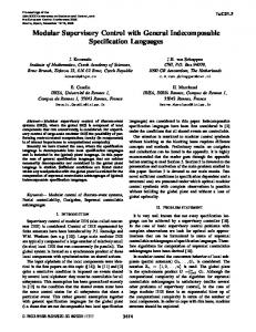
PC/104 computer, 500MHz PIII processor, with numerous I/O boards, running the QNX4.25 realtime operating system Wireless communications system (Orinoco 802.11b PCMCIA card), and antennas Forward looking sensors, including an Eaton-Vorad EVT-300 Doppler radar and a Denso lidar Accelerometers Yaw-rate gyroscope Stock engine control module WABCO braking system Magnetometers Steering actuator Power electronics.

The real-time software for the buses was written using the TejaNP software platform [29]. TejaNP is a development environment for system design and validation, optimized code generation, testing and debugging. TejaNP provides both a graphical application development environment, and a runtime system. The development process is as follows: specification of modular application data structures and program logic, placement of these application components in software architectures, mapping of the software architectures onto userspecified hardware architectures (there may be several processors), and finally automated code generation and debugging.

VIII. EXPERIMENTAL RESULTS The demonstration occurred on August 23 and 24, on a portion of I-15 in San Diego running roughly between the Miramar Naval-Air Station and the road to Poway. The test track is a reversible commuter lane made available to Berkeley for testing in the evenings of weekdays and on the weekends. The lanes are made available by CalTrans, who also provides assistance with the operation of the lanes. Also, controllers not developed by the authors were displayed to perform bus precision docking and lane tracking. A. Experimental Platform Three modified transit buses were at our disposal for experimental testing. Two of the buses were 40 foot long New Flyer buses, powered by CNG engines. The third bus was a 60 foot long articulated bus powered by a Detroit Diesel engine. For a complete description of the individual components installed, refer to [41]. A brief summary of the additional hardware include:

Figure 11. Hardware Setup on 40ft New Flyer Bus. B. Experimental Results The experimental results presented in this section involve a two-vehicle following scenario on I-15. A 40-foot CNG bus was driven automatically as a leading vehicle, and the

11

Next, Figure 13 shows an example of the closing and opening gap maneuvers. The relative inter-vehicle distance was decreased from 40 m to 20 m after about 210 seconds and increased back to 40 m after about 360 seconds. Plots (a) and (b) show the vehicle velocities and the velocity tracking error of the lead vehicle. The velocity tracking error of the lead vehicle stays less than 0.5 m/s, while the distance tracking error of the following vehicle is within 2 m as shown in plot (c). (a)

Speed (m/s)

25 20 15

v vdes

10 5 0

100

200

300 (b)

400

500

600

Range (m)

50 R Rdes

40 Switching manual to automatic driving

30 20 10 0

100

200

100

200

300 (c)

400

500

600

300

400

500

600

Distance error (m)

8 6 4 2 0 -2 0

Time (second)

Figure 12. Switching Manual to Automatic Driving and Distance Tracking: Driving Southbound on I-15.

v lead- vdes (m/s)

Speed (m/s)

(a)

Range (m)

automated 60-foot articulated bus followed with a given desired spacing. Plot (a) of Figure 12 below shows time responses of the two transit buses as well as a given desired speed profile with respect to time. For the given scenario, plots (b) and (c) show range and distance tracking error between two automated transit buses. Furthermore, the operating mode of both vehicles was switched from manual to automatic control at the approximate speed of 13 m/s via the DVI (after about 40 second in the figure). The following vehicle closed the distance from the initial separation to the desired distance of 15 m. It should be noted that there is a fairly steep hill during the period from 90 to 220 seconds, which results in larger distance tracking error (up to 2 m). Except for this period, the distance tracking error remains under 0.5 m during the constant distance following maneuver. It is suggested that some form of road grade estimation could improve the distance following performance in the presence of a steep grades.

20 vdes

10 0 0 0.5

vlead vfollow

100

200

100

200

(b)

300

400

500

0 -0.5 0 50

(c)

300

400

500

40 Rdes R1

30 20 0

100

200 300 Time (second)

400

500

Figure 13. Closing and Opening Gap Maneuver: Driving Southbound on I-15.

IX. CONCLUSIONS This paper presents a review of modeling, analysis and verification of complex systems and describes the use of a model-based approach to the development of real-time, embedded, hybrid control software for vehicle following and Bus Rapid Transit applications. The models and controllers that have been developed are public-domain and have been used by several leading universities and research groups; hopefully, those models or their future generations will continue to help bridge the chasm between model-based embedded systems theory and practice. The V2V libraries are available from: http://robotics.eecs.berkeley.edu/~anouck/mobies.html The Rapid Transit Bus platform was designed to provide realistically scaled embedded-system targets to test the application of MoBIES technologies to automotive control system development, in particular vehicle level coordination and control. We set up a vehicle platform, suited for robust, rapid prototyping approaches in design, testing, and implementation of embedded systems for transit buses under a varied set of conditions. The model-based process places strong emphasis on performing as much testing and verification in “tight-loops” as possible. Thus we hope to catch bugs early on in the development process and minimize cost associated with fixing the problems. Our models and controllers are framed in the context of hybrid automata. The use of a model with well-understood mathematical properties allows formal verification of the controller, and additional information about the experimental platform allows us to verify timing properties of the software. This gives us a high degree of confidence in the performance of the generated code. Experimental results involving two transit buses driving on a HOV lane of I-15 are presented.

12 REFERENCES [1] [2] [3] [4] [5]

[6] [7]

[8]

[9] [10]

[11]

[12] [13]

[14]

[15] [16] [17] [18]

[19]

[20]

[21]

[22]

[23]

[24]

[25]

[26]

N. Lynch, “Distributed Algorithms”, Morgan-Kaufman Publishers, Inc. San Mateo, CA, 1996. D. Harel, “Statecharts: A Visual Formalism for Complex Systems”, Science of Computer Programming, 8:231-274, 1987. N. Lynch, Class Notes, MIT, Computer Science Department class #6.879, 2001. B. Alpern and F.B. Schneider, “Recognizing Safety and Liveness”, Distributed Computing, 2 (3):117-126, 1987. B. Powel-Douglass, “Doing Hard Time: Developing Real-Time Systems with UML, Objects, Frameworks and Patterns”, Addison-Wesley Publishing Company, 1999. http://www.wikipedia.org/wiki/Embedded_system, from Wikipedia, the free Encyclopedia M. Drew and J.K. Hedrick, “A Discussion of Vehicle Modeling for Control”, Vehicle Dynamics Laboratory Technical Report, Mechanical Engineering Department, UC Berkeley. D. Cho and J.K. Hedrick, “Automotive Engine Modeling for Control”, ASME Journal of Dynamic Systems, Measurement and Control, December 1989, Vol. 111, pp. 568-576. www.timesys.com Franjo Ivancic, “Report on Verification of the MoBIES Vehicle-Vehicle Automotive OEP Problem”, Technical Report # MS-CIS-02-02, University of Pennsylvania, Philadelphia, PA, March 2002. N. Shankar, S. Owre and J. Rushby, “The PVS Proof-Checker: A Reference Manual”, Technical Report, Computer Science Lab, SRI International, Menlo Park, CA 1993. S.J. Garland and J.V. Guttag, LP, The Larch Prover, http://www.sds.mit.edu/~garland/LP/overview.html E.M. Clarke, O. Grumberg and D.E. Long, “Model Checking and Abstraction”, ACM Transactions on Programming Languages and Systems, 16 (5):1512-, September 1994. M. Abadi and L. Lamport, “Composing Specifications”, ACM Transactions on Programming Languages and Systems, 15 (1):73-132, January 1993. R. Milner, “Communicating and Mobile Systems: The Pi-Calculus”, Cambridge University Press, 1999. Z. Manna and A. Pnueli, “Temporal Verification of Reactive Systems: Safety”, Springer-Verlag, New York, 1995. S. Yovine, “Model Checking Timed Automata”, Lectures on Embedded Systems, LNCS Volume 1494, October 1998. Y. Kesten, Z. Manna and A. Pnueli, “Verification of Clocked and Hybrid Systems”, Lectures on Embedded Systems, LNCS Volume 1494, October 1998. R. Alur and C. Coucourbetis, N. Halbwachs, T.A. Henzinger, P.H. Ho, X. Nicollin, A. Olivero, J. Sifakis, and S. Yovine, “The Algorithmic Analysis of Hybrid Systems”, Theoretical Computer Science, 138 (1):334, 1995. N. Lynch, R. Segala and F. Vaandraager, “Hybrid I/O Automata Revisited”, Fourth International Workshop on Hybrid Systems, Computation and Control (HSCC), LNCS Volume 2034, SpringerVerlag, 2001. Rajeev Alur, Radu Grosu, Yerang Hur, Vijay Kumar, and Insup Lee, “Modular Specifications of Hybrid Systems in CHARON”, Hybrid Systems: Computation and Control, LNCS Volume 1790, pp. 6-19, 2000. A. Chutinan and B. H. Krogh, “Computational Techniques for Hybrid System Verification”, IEEE Transactions on Automatic Control, 48 (1):64-75, 2003. Ashish Tiwari, "Approximate Reachability for Linear Systems", Proceedings of Hybrid Systems: Computation and Control (HSCC), LNCS Volume 2623, Springer-Verlag, 2003. A.B. Kurzhanski, P. Varaiya, “Ellipsoidal Techniques for Reachability Analysis”, Proceedings of Hybrid Systems: Computation and Control (HSCC), LNCS Volume 1790, Springer-Verlag, 2000. T.A.Henzinger, P.H. Ho and H. Wong-Toi, “Hy-Tech: A Model Checker for Hybrid Systems”, Software Tools for Technology Transfer, 1:110122, 1997. M. Branicky, “Studies in Hybrid Systems: Modeling, Analysis and Control”, Ph. D. Thesis, EECS, MIT, Cambridge, MA, 1995.

[27] John Lygeros, Claire Tomlin and Shankar Sastry, “Controllers for Reachability Specifications for Hybrid Systems", Automatica, Special Issue on Hybrid Systems, March 1999, pp. 349-370 [28] http://www.mathworks.com/access/helpdesk/help/toolbox/stateflow/state flow.shtml [29] http://www.teja.com [30] http://www.fta.dot.gov/research/fleet/brt/brt.htm [31] A. Girard, J. Sousa and J.K. Hedrick, “A Hierarchical Control Architecture for the Mobile Offshore Base”, Marine Structures Journal, Vol. 13, No. 4-5, July 2000, pp.459-476. [32] A. Girard, J. Sousa, J. Misener and J.K. Hedrick, "A Control Architecture for Integrated Cooperative Cruise Control and Collision Warning Systems", Proceedings of the IEEE Conference on Decision and Control, 2001, Orlando, Florida, December 2001. [33] P. Varaiya, "Smart Cars on Smart Roads: Problems of Control", IEEE Transactions on Automatic Control, Vol. 38, No. 2, February 1993. [34] M. Broucke and P. Varaiya, ‘’The Automated Highway System: A Technology for the 21st Century’’, Control Engineering Practice, Vol. 5, No. 11, pp. 1583-90, 1997. [35] F. Eskafi, D. Khorrambadi, and P. Varaiya, "SmartPath: An Automated Highway System Simulator", Tech. Rep. PATH Tech. Memo 92-3, Institute of Transportation Studies, University of California, Berkeley, CA 94720, October 1992. [36] A. J. Healey, D.B. Marco and R. B. McGhee, Autonomous Underwater Vehicle Control Coordination Using A Tri-Level Hybrid Software Architecture, Proc. of 1996 IEEE Conference on Robotics and Automation, Minneapolis, Minnesota, April 1996, pp 2149-2159. [37] A. Girard, "A Convenient State Machine Formalism for High-Level Control of Autonomous Underwater Vehicles", Master’s Thesis, Florida Atlantic University, Boca Raton, FL, May 1998. [38] D. N. Godbole, J. Lygeros and S. Sastry, "Hierarchical Hybrid Control: An IVHS Case Study", in Hybrid Systems II (P. Antsaklis, A. Nerode and S. Sastry, eds.), no 999 in LNCS, Springer Verlag, 1995. [39] B. Song, J.K. Hedrick, and A. Howell, Fault tolerant control and classification for longitudinal vehicle control, Journal of Dynamic Systems, Measurement, and Control, vol. 125, September, 2003, pp 320-329. [40] A. Howell, B. Song, and J.K. Hedrick, Cooperative range estimation and sensor diagnostics for vehicle control, Proceedings of ASME: Dynamic Systems and Control Division, Nov. 2003. [41] Development and Demonstration of Automated Bus Rapid Transit and Automated Truck Operations, California PATH Technical Report, 2003. [42] R. W. D. Nickalls, 1993, “A new approach to solving the cubic: Cardan’s solution revealed,” The Mathematical Gazette, vol. 77, pp. 354-360.

ACKNOWLEDGMENTS The authors wish to acknowledge funding from DARPA/ITO under Grant F33615-00-C-1698 (MoBIES), and from CalTrans and California PATH under Task Orders 4228 and 4229. The authors would like to thank Anupam Pathak, who implemented the simplified V2V libraries in TEJA as part of his work on the MoBIES project in the summer of 2002, and BongSob Song, a fellow post-doctoral researcher who designed the low-level controller for the bus demonstration and participated in many joint data collection experiments. Bus poster is courtesy of Daniel Schickele. Anouck R. Girard received her Diplôme d’Ingénieur from the École des Mines d’Alès, France in 1993, her Master’s of Science from Florida Atlantic University, Boca Raton, FL in 1998, and her Ph.D. from the University of California, Berkeley in 2002, all of them in engineering. She was a Visiting Post-Doctoral Researcher at the University of California, Berkeley from 2002 to 2004 and is now an Assistant Professor of Mechanical Engineering at Columbia University, New York, NY. She has taught classes at Berkeley on automatic control theory. Her research interests include systems engineering with applications to intelligent systems, hybrid, distributed and embedded systems, autonomous vehicles, mobile, air and

13 ocean robots, mixed initiative, supervisory control and non-linear and sliding mode control. Prof. Girard is a member of Phi Kappa Phi, and the recipient of the ASME Best Student Paper Award in the OOAE division in 2001. Adam S. Howell received the B.S. degree in aerospace engineering from the University of Maryland, College Park, in 1996, and the Ph.D. degree in mechanical engineering from the University of California, Berkeley, in 2002. He was a Visiting Post-Doctoral Researcher at the University of California, Berkeley from 2002 to 2004 and is now a Senior Research Scientist with Lockheed Martin’s Advanced Technology Center. His research interests include fault diagnostics, sensor fusion, nonlinear control, observer design and wireless communications, with applications to intelligent vehicles and UAVs. Dr. Howell is a member of Sigma Gamma Tau and the Order of the Engineer.

J. Karl Hedrick received the B.S. degree from the University of Michigan, Ann Arbor, in 1966, and the M.S. and Ph.D. degrees from Stanford University, Stanford, CA, in 1970 and 1971, respectively. He was a Professor of Mechanical Engineering at the Massachusetts Institute of Technology, Cambridge, from 1974 to 1988, where he served as Director of the Vehicle Dynamics Laboratory. He is currently the James Marshall Wells Professor and Chairman of Mechanical Engineering at the University of California (UC), Berkeley. He teaches graduate and undergraduate courses in automatic control theory and vehicle dynamics. His research has concentrated on the development of advanced control theory and on its application to a broad variety of transportation systems including automated highway systems, collision warning systems, collision avoidance systems, and adaptive cruise control systems. His work has also included brake control and electronic suspension systems. The active suspension laboratory at UC Berkeley is the only full scale, half car test facility in the United States. He has also worked in the powertrain control area including engine and transmission control. He has offered short courses on active and semi-active suspensions, nonlinear control theory and VHS in the United States and in Europe. Prof. Hedrick has served on many national committees including the Transportation Research Board, the American National Standards Institute, ISO (International Standards Organization) and the NCHRP (National Cooperative Highway Research Program). He is currently a member of the Board of Directors and is Vice President of the International Association of Vehicle System Dynamics (IAVSD) and is the editor of the Vehicle Systems Dynamics Journal. He is a Fellow of ASME where he has served as Chairman of the Dynamic Systems and Controls Division and as Chairman of the Honors Committee. He is also a member of SAE.