Proceeding Series of the Brazilian Society of Applied and Computational Mathematics, Vol. 4, N. 1, 2016. Trabalho apresentado no DINCON, Natal - RN, 2015.
Proceeding Series of the Brazilian Society of Computational and Applied Mathematics
Hybridization of IMC and PID Control Structures from Filtered Positional Generalized Predictive Controller Rejane de Barros Ara´ ujo1 Daniel Cavalcanti Jeronymo2 Antonio Augusto Rodrigues Coelho3 Federal University of Santa Catarina Department of Automation and Systems 88040-900 Florianopolis, SC, Brazil
Abstract. The purpose of this paper is to derive an alternative tuning design from Generalized Predictive Controller (GPC) that is based on both positional plant model and cost function, involving the selection of an integral polynomial weighting filter. The obtained Filter Positional GPC can be transformed into RST structure and next to Filtered Internal Model and PID controllers. Numerical and experimental essays show the effectiveness of the control methodologies. Keywords. predictive control, PID controller, tuning, target tracking, stability analysis.
1
Introduction
The Generalized Predictive Controller (GPC) has been successfully implemented in several applications, showing good robustness, performance and dynamic stability [2, 4]. Hybridization of GPC to the Internal Model Control (IMC) structure has stimulated academia studies. However, few discrete implementations have been explored and aimed to extract the characteristics and advantages of the GPC to IMC in order to deal with a variety of complex processes and disturbance rejection. The work proposed in [5] has shown the GPC design with different types of constraints relating to the IMC control law, inserting anti-windup technique in numerical simulation scenarios. On the other hand, Proportional-Integral-Derivative (PID) controllers are widely used in the industry as standalone equipment or in CLP. The pioneer work using PID in the structure I+PD controller hybridized with GPC was proposed in [6], using a design method of a self-tuning PID controller. Next, [8] has extended the work of [6], inserting a filter in the reference of the GPC law, where the PID controller has a filter to tune the integral time of the controller. 1
[email protected] [email protected] 3
[email protected] 2
DOI: 10.5540/03.2016.004.01.0013
010013-1
© 2016 SBMAC
Proceeding Series of the Brazilian Society of Applied and Computational Mathematics, Vol. 4, N. 1, 2016.
2 The purpose of this paper is to derive a design alternative for the GPC synthesis, from a positional plant model, involving the selection of an integral polynomial weighting factor for reference and plant output signals. This control scheme is called filtered positional GPC (FP-GPC). The FP-GPC is transformed into two degree of freedom polynomial RST structure and next to Filtered Internal Model (F-IMC) and PID controllers. The idea is to inherit the FP-GPC properties (stability, uncertainty, setpoint tracking) to the PID and F-IMC control structures, investigating applications in different types of plants. This paper is organized as follows: Section 2 presents briefly the FP-GPC design. Sections 3 and 4 describe how the FP-GPC controller, in the RST form, is convert to F-IMC and PID control schemes, respectively. Numerical and practical simulations are also included. Finally, conclusions are given in Section 5.
2
Filtered Positional GPC Design
Consider the deterministic CAR model (Controlled Auto-Regressive) of the controlled plant characterized by the following positional discrete transfer function: A(q −1 )y(t) = q −d B(q −1 )u(t − 1)
(1)
where y(t) is the process output, u(t) is the control signal, d is the dead-time and the roots of the polynomials A(q −1 ) and B(q −1 ) characterize the open-loop poles and zeros, respectively. The GPC control law is obtained by minimizing the cost function given by Ny Nu X X J= {φy (t + j) − φw (t + j)}2 + λ u2 (t + j − d − 1) j=1
(2)
j=1
with φy (t + j) and φw (t + j) auxiliary output and reference variables and are defined as φy (t) = P (q −1 )y(t) =
Kα α(q −1 ) y(t) ∆
,
φw (t) = P (q −1 )w(t) =
Kα α(q −1 ) w(t) ∆
(3)
where w(t) is the setpoint, ∆ = (1 − q −1 ), λ is the control weighting, Ny is the output prediction horizon and Nu is the control horizon. Polynomials P (q −1 ) and α(q −1 ) are correlated with closed-loop system dynamic and filtering aspects, respectively, and Kα represents the filter gain. The term φy (t + j) is replaced by the estimated value, the equation (1) is multiplied by P (q −1 ) and can be rewritten as ∆A(q −1 )φy (t + j) = Kα α(q −1 )B(q −1 )u(t + j − d − 1) The minimization of the cost function generates the FP-GPC for the unconstrained case, and the control vector is calculated by U = (GT G + λI)−1 GT [Φw − Φf ]
DOI: 10.5540/03.2016.004.01.0013
010013-2
(4)
© 2016 SBMAC
Proceeding Series of the Brazilian Society of Applied and Computational Mathematics, Vol. 4, N. 1, 2016.
3 which is a similar formalism of the incremental GPC design of [2] for the incremental fixed structure. To analyze the influence of the filter P (q −1 ) for setpoint changes and disturbance attenuation control purposes, the equation (4) can be rewritten to the polynomial RST canonical form such as Ny Ny Ny X X X j 1 + q −1 kj Gj u(t) = kj q φw (t) − kj Fj φy (t) (5) j=1
j=1
j=1
where K is the vector obtained from the first row of the matrix (GT G + λI)−1 GT . Next, using the definition of P (q −1 ), then the RST canonical structure of the FP-GPC is given by R(q −1 )∆u(t) = Kα α(q −1 )T (q −1 )w(t) − Kα α(q −1 )S(q −1 )y(t) (6) The block diagram of the RST structure for the FP-GPC design is shown in Figure (1). Reference, output and control filters are observed in a two degree of freedom control scheme, where R(q −1 ) and S(q −1 ) are designed to obtain the desired regulatory performance (disturbance rejection) and T (q −1 ) is designed to guarantee reference tracking (both polynomials depend on how the tuning parameters of the FP-GPC are selected).
Figure 1: Disturbance on the input and output under FP-GPC system diagram. Although not shown, it is important to say that for all simulation results of this paper, the filter parameters Kα and α(q −1 ) of the FP-GPC are calibrated through a multi∆
objective optimization algorithm based on the sensitivity function (Ms = max |A(e−jω ) 0≤ω